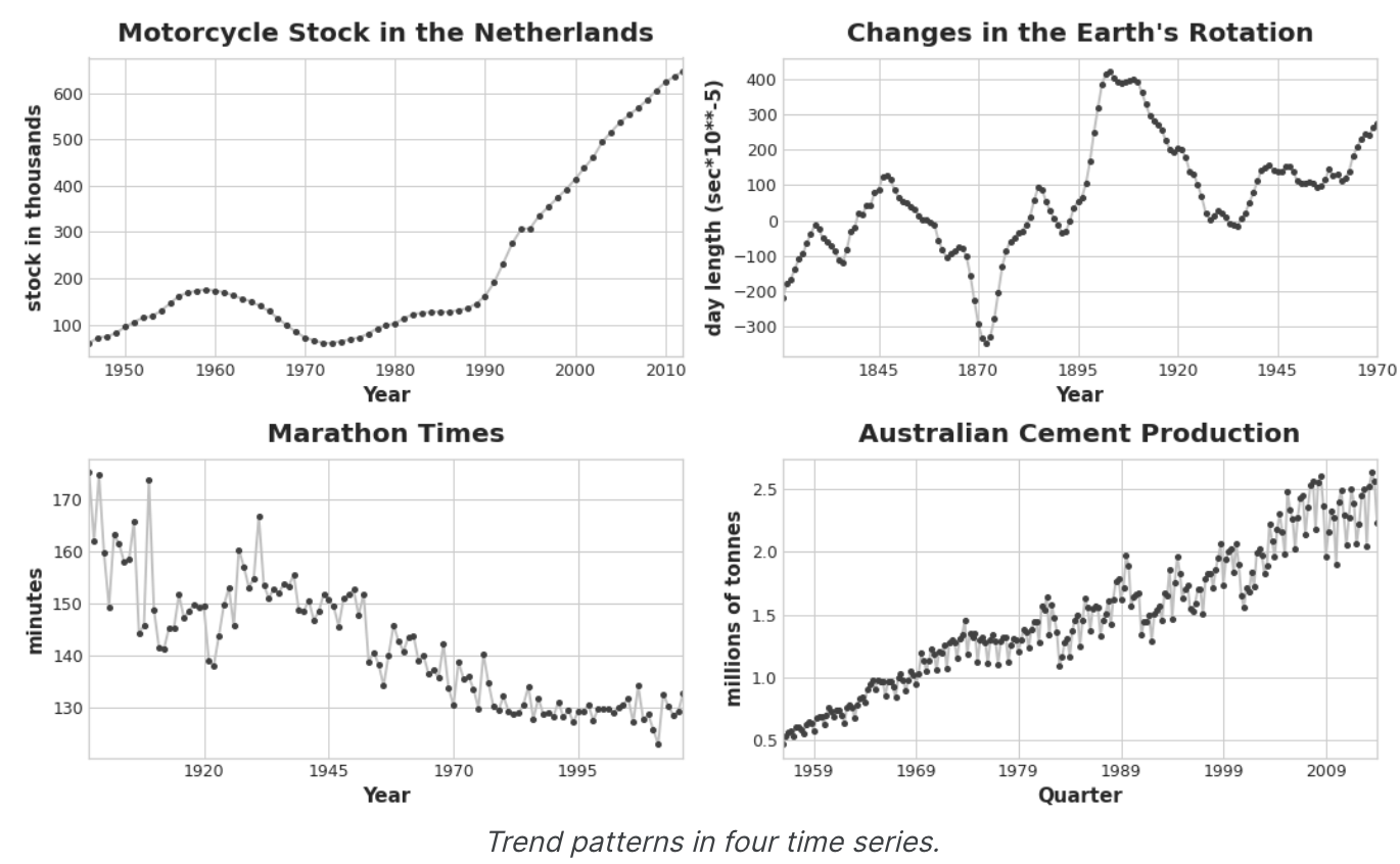
What is Trend?

시계열의 추세 구성 요소는 시계열 평균의 지속적이고 장기적인 변화를 나타낸다. 추세는 시계열에서 가장 느리게 움직이는 부분으로, 가장 중요한 시간 규모를 나타내는 부분이다. 제품 판매량의 시계열에서 추세가 증가하는 것은 해마다 더 많은 사람들이 제품을 알게되면서 시장이 확장되는 효과 일 수 있다.

이 코스에서는 평균의 추세에 초점을 맞춘다고 함.

Moving Average Plots

시계열의 평균을 확인하려면 이동 평균 차트(Moving Average Plots)를 사용할 수 있다. 시계열의 이동 평균을 계산하려면 정의된 폭의 슬라이딩 창 내에 있는 값의 평균을 계산한다.
그래프의 각 점은 양쪽 창 안에 있는 시계열의 모든 값의 평균을 나타낸다. 이 개념은 시계열의 단기 변동을 완화하여 장기적인 변화만 남도록 하는 것이다.

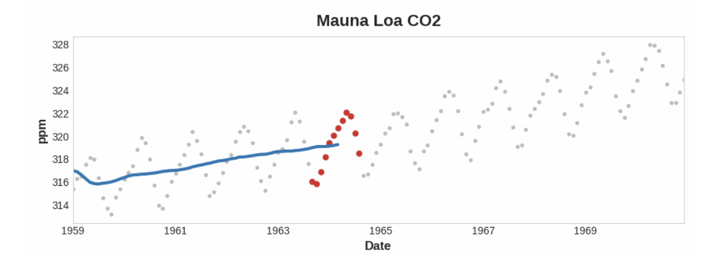
A moving average plot illustrating a linear trend. Each point on the curve (blue) is the average of the points (red) within a window of size 12

위의 Mauna Loa 시리즈에서 해마다 위 아래로 반복되는 움직임, 즉 단기적인 계절적 변화를 확인할 수 있다. 변화가 추세의 일부가 되려면 계절적 변화보다 더 긴 기간에 걸쳐 발생해야 한다. 따라서 추세를 시각화하려면, 시리즈의 계절적 기간보다 긴 기간의 평균을 취한다. Mauna Loa의 경우 각 연도의 계절을 부드럽게 표현하기 위해 12 크기의 창을 선택했다.

Engineering Trend

추세의 형태 파악 -> Time-step features를 활용하여 모델링 시도
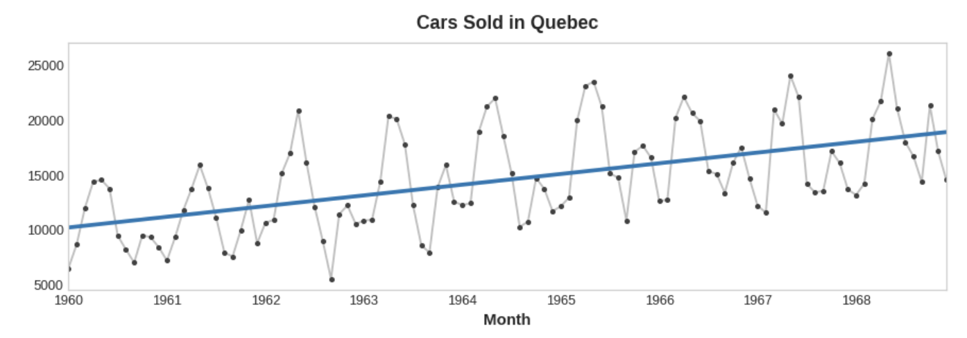
시간 더미 자체를 사용하여 선형 추세를 모델링하는 방법은 이미 살펴 봤다.

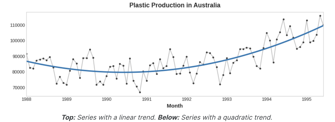
target = a * time + b

시간 더미의 변환을 통해 다른 많은 종류의 추세를 맞출 수 있다. 추세가 이차 함수(포물선)인 것 처럼 보이면 시간 더미의 제곱을 기능 집합에 추가하기만 하면 된다.

target = a * time ** 2 + b * time + c

선형 회귀는 계수 a, b, c를 학습한다.

아래 그림의 추세 곡선은 이러한 종류의 기능과 scikit-learn의 LinearRegression을 사용하여 fit 했다.

Example - Tunnel Traffic

이 샘플에서는 추세 모델을 만들 것임

from pathlib import Path
from warnings import simplifier

import matplotlib.pyplot as plt
import numpy as np
import pandas as np

simplifier("ignore")
# Set Matplotlib defaults
plt.style.use("seaborn-whitegrid")
plt.rc("figure", autolayout=True, figsize=(11, 5))
plt.rc(
    "axes",
    labelweight="bold",
    labelsize="large",
    titleweight="bold",
    titlesize=14,
    titlepad=10,
)
plot_params = dict(
    color="0.75",
    style=".-",
    markeredgecolor="0.25",
    markerfacecolor="0.25",
    legend=False,
)
%config InlineBackend.figure_format = 'retina'

# Load Tunnel Traffic dataset
tunnel = pd.read_csv(filepath, parse_dates=["Day"])
tunnel = tunnel.set_index("Dat").to_period()

parse_dates : DD/MM/YYYY 의 형태를 보기 쉽게 YYYY-MM-DD 형태로 바꿔줌

to period() : DataTimeIndex나 Series를 주기 기반의 PeriodIndex 로 바꾸어 줌

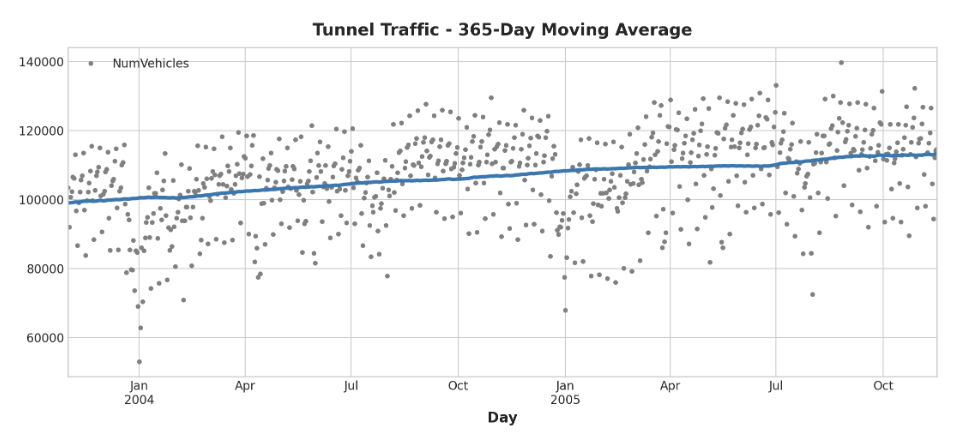
이동 평균 plot을 만들어 이 계열이 어떤 Trend를 가지고 있는지 확인해보자.
daily observation이므로, 1년 이내의 단기적인 변화를 부드럽게 처리하기 위해 365일 기간을 선택

이동 평균을 만드려면 먼저 rolling method를 사용하여 윈도우 계산을 시작한다. 그런 다음 mean method를 사용하여 해당 기간 동안의 평균을 계산한다.
터널 그래픽의 추세는 선형에 가까운 것으로 보인다.

moving_average = tunnel.rolling(
	window=365, 		# 365-day window
    center=True, 		# puts the average at the center of the window
    min_periods=183, 	# choose about half the window size
).mean() 				# compute the mean (could also do median, std, min, max etc)

ax = tunnel.plot(style=".", color="0.5")
moving_average.plot(
	ax=ax, linewidth=3, title="Tunnel Traffic - 365-Day Moving Average", legend=False,
);

1강에서는 pandas에서 Time Dummy를 직접 생성했지만, 이제부터 통계 모델 라이브러리에서 DeterministicProcess라는 함수를 사용한다.
이 함수를 사용하면 시계열 및 선형 회귀에서 발생할 수 있는 몇 가지 까다로운 실패 사례를 피할 수 있다.
순서 인수는 다항식 순서를 나타낸다.

• 1은 선형, 2는 2차, 3은 3차 등 다항식 순서를 나타냄

from statsmodels.tsa.deterministic import DeterministicProcess

dp = DeterministicProcess(
	index=tunnel.index,			# dates from the training data
    constant=True,				# dummy features for the bias (y_intercept)
    order=1,					# the time dummy (trend)
    drop=True					# drop terms if necessary to avoid collinearity(선형성)
)

# 'in_sample' creates features for the dates given in the 'index' argument
# in_sample은 index 인수에 지정딘 날짜에 대한 feature를 생성
X = dp.in_sample()

X.head()

(deterministic process는 구성 및 시계열과 같이 무작위가 아니거나 완전히 결정된 시계열을 나타내는 기술 용어이다. 시간 인덱스에서 파생된 특징은 일반적으로 deterministic하다고 할 수 있다.)

기본적으로 이전과 동일하게 trend model을 만들지만, fit_intercept=False 인수를 추가

from sklearn.linear_model import LinearRegression

y = tunnel["NumVehicles"] 			# the target

# the intercept is the same as the 'const' feature from
# DeterministicProcess. LinearRegression behaves badly with duplicated
# features, so we need to be sure to exclude it here
# intercept(절편)를 제외해야한다는 의미

model = LinearRegression(fit_intercept=False)
model.fit(X, y)

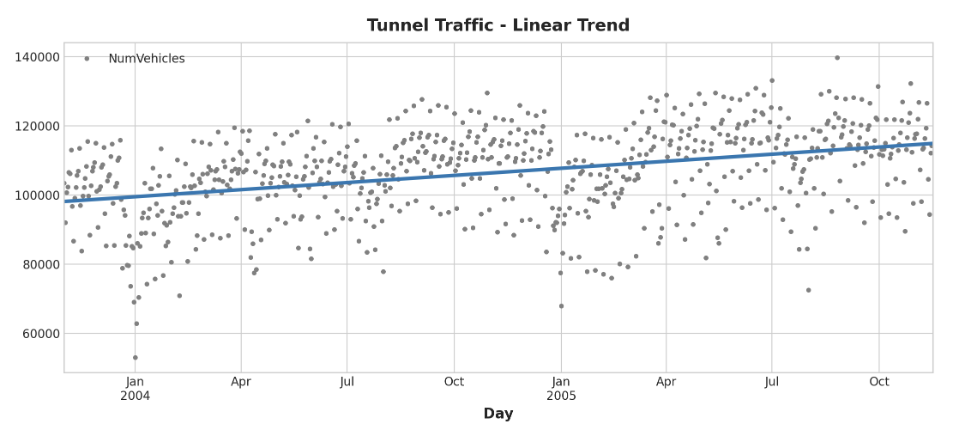
y_pred = pd.Series(model.predict(X), index=X.index)

선형 회귀 모델에서 발견한 Trend는 이동 평균 plot과 거의 동일하므로, 이 경우 선형 Trend가 올바른 결정이었음을 시사함

ax = tunnel.plot(style=".", color="0.5", title="Tunnel Traffic - Linear Trend")
_ = y_pred.plot(ax=ax, linewidth=3, label="Trend")

(_는 의미없는 반환 값을 처리하기 위한 장치, return 0; 느낌)

예측을 하기 위해 "표본 외(out of sample)" 특징에 모델을 적용한다. "표본 외"는 학습 데이터의 관찰 기간을 벗어난 시간을 의미한다. 30일 예측을 만드는 방법은 다음과 같음

X = dp.out_of_sample(steps=30)

y_fore = pd.Series(model.predict(X), index=X.index)

y_fore.head()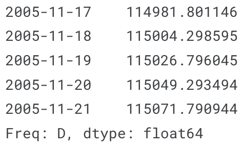

시리즈의 일부를 plot하여 향후 30일 동안의 Trend 예측을 확인

ax = tunnel["2005-05":].plot(title="Tunnel Traffic - Linear Trend Forecast", **plot_params)
ax = y_pred["2005-05":].plot(ax=ax, linewidth=3, label="Trend")
ax = y_fore.plot(ax=ax, linewidth=3, label="Trend Forecast", colot="C3")
_ = ax.legend()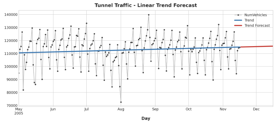

이 단원에서 배운 Trend 모델은 유용하고 트렌드를 학습할 수 없는 알고리즘(XGBoost, RandomForest)을 사용하는 Hybrid model의 구성요소로도 사용할 수 있따.