Combine the strengths of two forecasters with this powerful technique.

Introduction

선형 회귀는 추세를 추정하는 데는 탁월하지만 상호 작용을 학습할 수는 없다. XGBoost는 상호작용을 학습하는 데는 탁월하지만 추세를 추정할 수는 없다.
이 단원에서는 상호 보완적인 학습 알고리즘을 결합하여 한 알고리즘의 강점이 다른 알고리즘의 약점을 보완하는 "하이브리드" 예측기를 만드는 방법에 대해 알아보자.

Components and Residuals (구성 요소 및 잔여물)

효과적인 하이브리드를 설계하려면 시계열이 어떻게 구성되는지 더 잘 이해해야 한다.
지금까지 추세, 계절, 주기의 세 가지 의존성 패턴을 배웠다.
많은 시계열은 이 세 가지 구성 요소와 본질적으로 예측할 수 없는 완전히 무작위적인 오류를 더한 모델로 자세히 설명할 수 있다.

series = trend + seasons + cycles + error

그러면 이 모델의 각 항을 시계열의 구성 요소(components)라고 부를 수 있다.

모델의 잔차(residual)은 모델이 학습된 대상과 모델이 예측한 것 사이의 차이, 즉 실제 곡선과 적합 곡선 사이의 차이이다. residual을 특징에 대해 plot하면 대상에서 "남은" 부분, 즉 모델이 해당 특징에서 대상에 대해 학습하지 못한 부분을 얻을 수 있다.

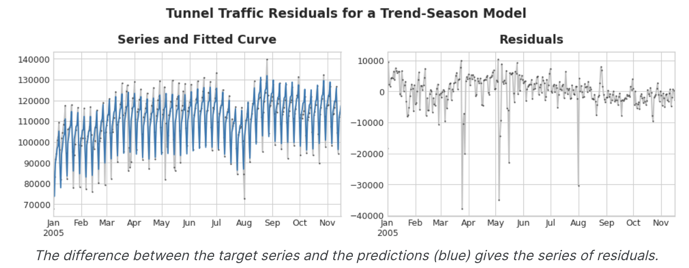
위 그림의 왼쪽에는 터널 교통량 계열의 일부와 Trend-Seasonal 곡선이 있다.
적합 곡선을 빼면 오른 쪽에 residual이 남는다. residual에는 Trend-seasonal 모델이 학습하지 못한 터널 교통량의 모든 것이 포함되어 있다.

시계열의 구성 요소를 학습하는 것은 반복적인 과정으로 상상할 수 있다.

• 먼저 추세를 학습하여 시계열에서 빼고
• detrended residual(탈추세 잔차)에서 계절성을 학습하여 계절을 빼고
• 주기를 학습하여 주기를 빼고
• 마지막으로 예측할 수 없는 오차만 남게 된다.
  
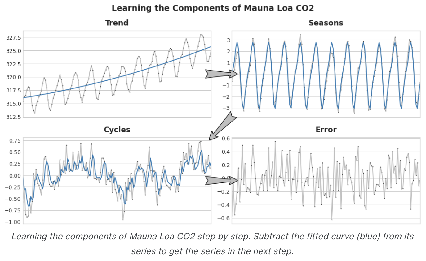
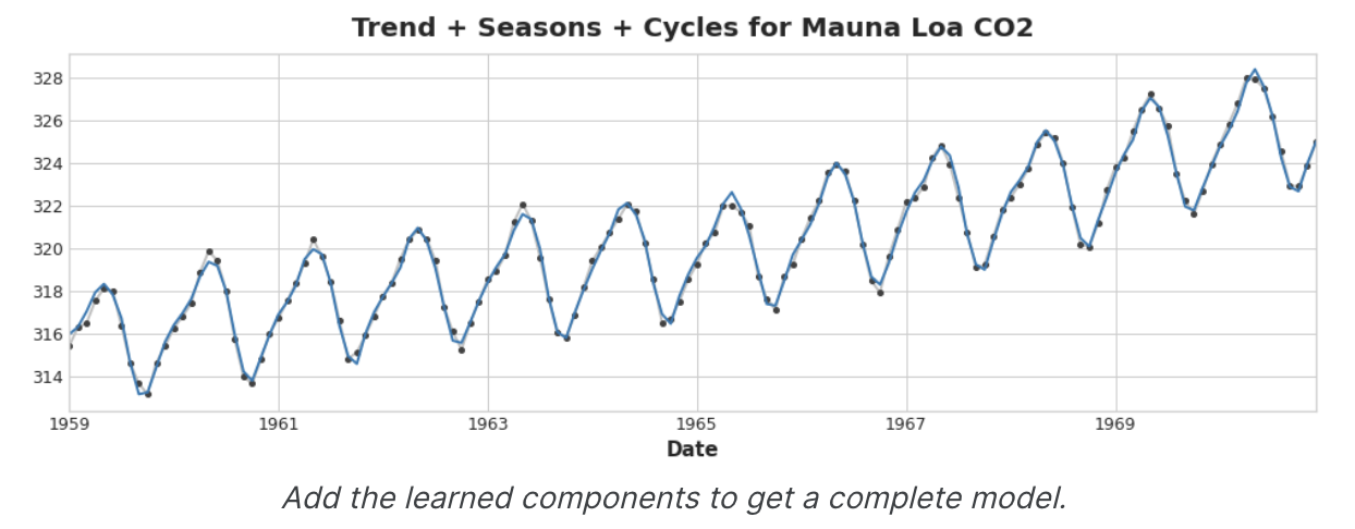
  학습한 모든 구성 요소를 더하면 완전한 모델을 얻을 수 있다.
  추세, 계절, 주기를 모델링하는 전체 기능 집합에 대해 선형회귀를 학습시킨다면 이러한 작업을 수행할 수 있다.
  

Hybrid Forecasting with Residuals

이전 단원에서는 단일 알고리즘(선형 회귀)을 사용하여 모든 구성 요소를 한 번에 학습했다. 하지만 일부 구성 요소에는 하나의 알고리즘을 사용하고 나머지 구성 요소에는 다른 알고리즘을 사용할 수도 있다. 이렇게 하면 항상 각 구성 요소에 가장 적합한 알고리즘을 선택할 수 있다.이를 위해 하나의 알고리즘을 사용하여 원래 시리즈에 맞추고 두 번째 알고리즘을 사용하여 나머지 시리즈에 마주는 것이다.

상세 프로세스는 다음과 같음.

# 1. Train and predict with first model
model_1.fit(X_train_1, y_train)
y_pred_1 = model_1.predict(X_train)

# 2. Train and predict with second model on residuals
model_2.fit(X_train_2, y_train - y_pred_1)
y_pred_2 = model_2.predict(X_train_2)

# 3. Add to get overall predictions
y_pred = y_pred_1 + y_pred_2

의외로 간단하네?

일반적으로 각 모델에서 학습하고자 하는 내용에 따라 서로 다른 기능 세트(위의 X_train_1 및 X_train_2)를 사용하고자 한다.
예를 들어 첫 번째 모델을 사용하여 트렌드를 학습하는 경우 일반적으로 두 번째 모델에는 Trend Feature가 필요하지 않다.

두 개 이상의 모델을 사용할 수는 있지만, 실제로는 특별히 도움이 되지 않는 것 같다고 함.
실제로 하이브리드를 구성하는 가장 일반적인 전략은 방금 설명한 것과 같이 간단한(보통 선형) 학습 알고리즘에 이어 GBDT나 심층 신경망과 같은 복잡한 비선형 학습자를 사용하는 것이다. 간단한 모델은 일반적으로 뒤에 나오는 강력한 알고리즘을 위한 '도우미'로 설계된다.

Design Hybrids

이 단원에서 설명한 방법 외에도 ML 모델을 결합하는 방법은 여러가지가 있음

회귀 알고리즘이 예측을 할 수 있는 방법에는 일반적으로 특징을 변환하거나 대상을 변환하는 두 가지 방법이 있다.
특징 변환 알고리즘은 특징을 입력으로 사용하는 수학적 함수를 학습한 다음, 이를 결합하고 변환하여 훈련 세트의 모고표 값과 일치하는 출력을 생성한다.
선형 회귀와 신경망이 이러한 종류의 알고리즘이다.

Target-transforming algorithms(목표 변환 알고리즘)은 feature를 사용하여 학습 집합의 목표 값을 그룹화하고 그룹 내 값의 평균을 구하여 예측을 수행하며, 특징 집합은 평균을 구할 그룹을 나타낼 뿐이다. Decision tree나 Nearest Neighbors가 이러한 알고리즘이다.

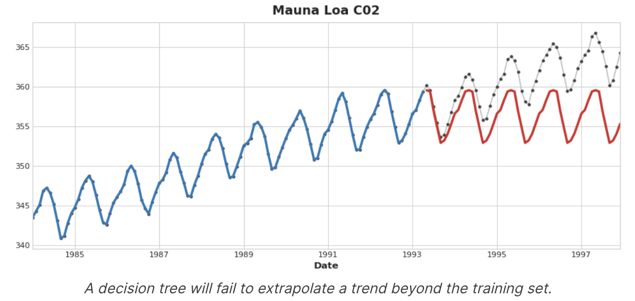
중요한 것은, feature transformers(특징 변환기)는 일반적으로 적절한 특징을 입력으로 주어지면 훈련 집합을 넘어 목표 값을 추정할 수 있지만, feature transformers의 예측은 항상 훈련 집합의 범위 내에 한정된다. time dummy가 time step을 계속 세는 경우 선형 회귀는 추세선을 계속 그린다. 동일한 시간 더미가 주어지면 의사 결정 트리는 학습 데이터의 마지막 단계가 나타내는 추세를 영원히 미래로 예측한다.
의사 결정 트리는 추세를 추정할 수 없다.
RandomForest나 Gradient Boost(like XGBoost)는 의사 결정 트리의 ensemble이므로 추세를 추정할 수 없다.

선형 회귀를 사용하여 추세를 추정하고, 대상을 변환하여 추세를 제거한 다음, detrended residual에 XGBoost를 적용하는 것이 이 단원에서 하이브리드 설계의 동기가 된다. 신경망(Feature transformer)을 하이브리드화 하려면 다른 모델의 예측을 특징으로 포함하는 대신 신경망이 자체 예측의 일부로 포함할 수 있다. residual에 fitting하는 법은 실제로 gradient boosting algorithm이 사용하는 방법과 동일하므로 이를 Boost Hybrid, 예측을 feature로 사용하는 방법은 stack 이라고 하며 이를 Stack Hybrid라고 한다.

Winning Hybrids from Kaggle Competitions
For inspiration, here are a few top scoring solutions from past competitions:
STL boosted with exponential smoothing - Walmart Recruiting - Store Sales Forecasting
ARIMA and exponential smoothing boosted with GBDT - Rossmann Store Sales
An ensemble of stacked and boosted hybrids - Web Traffic Time Series Forecasting
Exponential smoothing stacked with LSTM neural net - M4 (non-Kaggle)

Example - US Retail Sales

US Retail Sales 데이터셋에는 미국 인구조사국에서 수집한 1992년부터 2019년까지의 다양한 소매업에 대한 월별 판매 데이터가 포함되어 있다.
우리의 목표는 초기 연도의 매출을 바탕으로, 2016~2019년의 매출을 예측하는 것이다.
선형 회귀 + XGBoost 하이브리드를 만드는 것 외에도, XGBoost와 함께 사용하기 위해 시계열 데이터를 설정하는 방법도 살펴보자.

from pathlib import Path
from warnings import simplefilter

import matplotlib.pyplot as plt
import pandas as pd
from sklearn.linear_model import LinearRegression
from sklearn.model_selection import train_test_split
from statsmodels.tsa.deterministic import CalendarFourier, DeterministicProcess
from xgboost import XGBRegressor


simplefilter("ignore")

# Set Matplotlib defaults
plt.style.use("seaborn-whitegrid")
plt.rc(
    "figure",
    autolayout=True,
    figsize=(11, 4),
    titlesize=18,
    titleweight='bold',
)
plt.rc(
    "axes",
    labelweight="bold",
    labelsize="large",
    titleweight="bold",
    titlesize=16,
    titlepad=10,
)
plot_params = dict(
    color="0.75",
    style=".-",
    markeredgecolor="0.25",
    markerfacecolor="0.25",
)

data_dir = Path("../input/ts-course-data/")
industries = ["BuildingMaterials", "FoodAndBeverage"]
retail = pd.read_csv(
    data_dir / "us-retail-sales.csv",
    usecols=['Month'] + industries,
    parse_dates=['Month'],
    index_col='Month',
).to_period('D').reindex(columns=industries)
retail = pd.concat({'Sales': retail}, names=[None, 'Industries'], axis=1)

retail.head()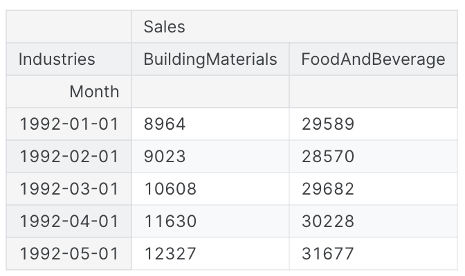

먼저 선형 회귀 모델을 사용하여 각 계열의 추세를 알아보자.
설명을 위해 이차(order 2) 추세를 사용한다.
적합도가 완전하지는 않겠지만 필요에 충분할 것이다.

y = retail.copy()

# Create trend features
dp = DeterministicProcess(
    index=y.index,  # dates from the training data
    constant=True,  # the intercept
    order=2,        # quadratic trend
    drop=True,      # drop terms to avoid collinearity
)
X = dp.in_sample()  # features for the training data

# Test on the years 2016-2019. It will be easier for us later if we
# split the date index instead of the dataframe directly.
idx_train, idx_test = train_test_split(
    y.index, test_size=12 * 4, shuffle=False,
)
X_train, X_test = X.loc[idx_train, :], X.loc[idx_test, :]
y_train, y_test = y.loc[idx_train], y.loc[idx_test]

# Fit trend model
model = LinearRegression(fit_intercept=False)
model.fit(X_train, y_train)

# Make predictions
y_fit = pd.DataFrame(
    model.predict(X_train),
    index=y_train.index,
    columns=y_train.columns,
)
y_pred = pd.DataFrame(
    model.predict(X_test),
    index=y_test.index,
    columns=y_test.columns,
)

# Plot
axs = y_train.plot(color='0.25', subplots=True, sharex=True)
axs = y_test.plot(color='0.25', subplots=True, sharex=True, ax=axs)
axs = y_fit.plot(color='C0', subplots=True, sharex=True, ax=axs)
axs = y_pred.plot(color='C3', subplots=True, sharex=True, ax=axs)
for ax in axs: ax.legend([])
_ = plt.suptitle("Trends")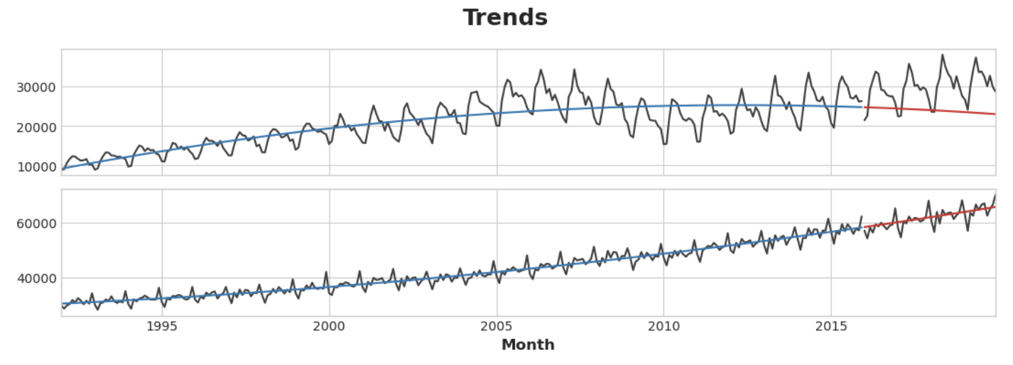

선형 회귀 알고리즘은 다중 출력 회귀가 가능하지만, XGBoost는 그렇지 않다. XGBoost를 사용하여 한 번에 여러 계열을 예측하려면 대신 column당 하나의 시계열이 있는 wide 형식에서 행을 따라 카테고리 별로 계열이 인덱싱되는 long format으로 변환한다.

# The 'stack' method converts column labels to row labels, pivoting from wide format to long
X = retail.stack()  # pivot dataset wide to long
display(X.head())
y = X.pop('Sales')  # grab target series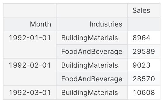

XGBoost가 두 시계열을 구분하는 방법을 학습할 수 있도록 'Industries' 행 레이블을 레이블 인코딩이 있는 categorical feature로 바꾼다. 또한 시간 인덱스에서 월 숫자를 가져와 연간 계절성을 나타내는 기능을 만든다.

# Turn row labels into categorical feauture columns with a label encoding
X = X.reset_index('Industries')
# Label encoding for 'Industries' feature
for colname in X.select_dtypes(["object", "category"]):
	X[colname], _ = X[colname].factorize()
    
# Label encoding for annual seasonality
X["Month"] = X.index.month # values are 1, 2, ...., 12

# Create splits
X_train, X_test = X.loc[idx_train, :], X.loc[idx_test, :]
y_train, y_test = y.loc[idx_train], y.loc[idx_test]

이제 앞서 만든 추세 예측을 long format으로 변환한 다음 원래 시리즈에서 뺀다.
이렇게 하면 XGBoost가 학습할 수 있는 Detrend(residual) series가 생성된다.

# Pivot wide to long (stack) and convert DataFrame to Series (squeeze)
y_fit = y_fit.stack().squeeze()    # trend from training set
y_pred = y_pred.stack().squeeze()  # trend from test set

# Create residuals (the collection of detrended series) from the training set
y_resid = y_train - y_fit

# Train XGBoost on the residuals
xgb = XGBRegressor()
xgb.fit(X_train, y_resid)

# Add the predicted residuals onto the predicted trends
y_fit_boosted = xgb.predict(X_train) + y_fit
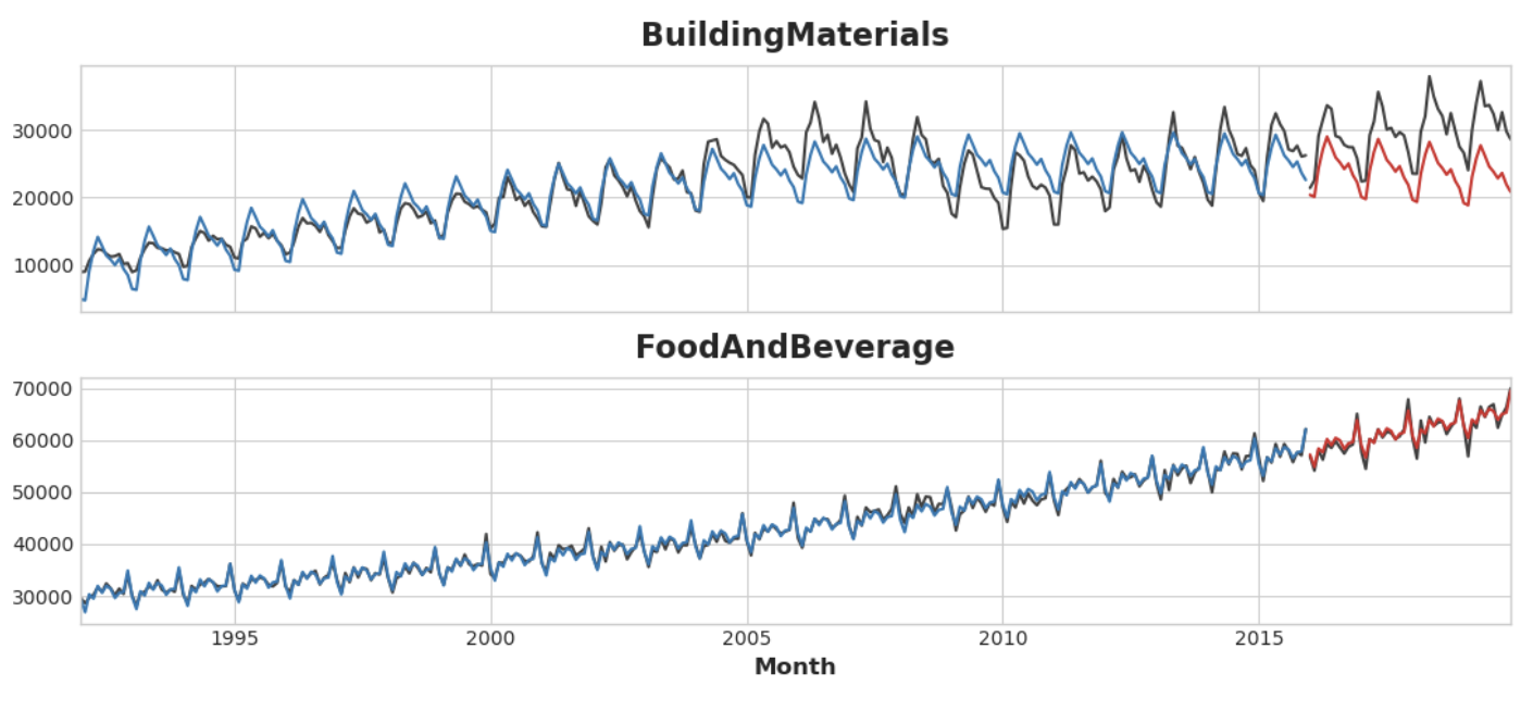
y_pred_boosted = xgb.predict(X_test) + y_pred

적합도는 상당히 좋은 것으로 보이나 XGBoost가 학습한 추세가 선형 회귀를 통해 학습한 추세만큼만 좋은 것을 볼 수 있으며, 특히 'BuildingMaterials' 시리즈에서 적합도가 좋지 않은 추세를 보완하지 못한 것을 알 수 있다.

axs = y_train.unstack(['Industries']).plot(
    color='0.25', figsize=(11, 5), subplots=True, sharex=True,
    title=['BuildingMaterials', 'FoodAndBeverage'],
)
axs = y_test.unstack(['Industries']).plot(
    color='0.25', subplots=True, sharex=True, ax=axs,
)
axs = y_fit_boosted.unstack(['Industries']).plot(
    color='C0', subplots=True, sharex=True, ax=axs,
)
axs = y_pred_boosted.unstack(['Industries']).plot(
    color='C3', subplots=True, sharex=True, ax=axs,
)
for ax in axs: ax.legend([])