• 논문제목: Improved Techniques for Grid Mapping with Rao-Blackwellized Particle Filters
• 발표 학회 및 년도: IEEE Transactions on Robotics, 2007

Overview of gMapping

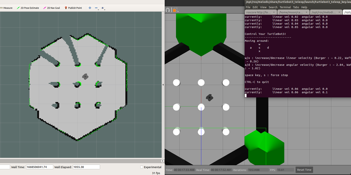
• gMapping SLAM은 ROBOTIS turtlebot3 SLAM 패키지에 default로 설정되어 있습니다
• gMapping SLAM은 가장 보편적으로 사용되는 SLAM 알고리즘이라 할 수 있습니다
• OpenSLAM에 의해 개발되었습니다.
• Rao-Blackwellization particle filter 기반의 Grid-based SLAM 방법입니다. 따라서 robot의 pose와 landmarks을 각각 추정하게 됩니다
• Laser-Range Sensor Data와 Odometry measurement를 사용하게 됩니다.
• 주변 환경이 static할 때 잘 작동한다고 합니다.

Problem Definition

• Given
  1) Observations: $z_{1:t} = z_{1}, ..., z_{t}$
  2) Odometry measurements: $u_{1:t} = u_{1}, ..., u_{t}$

• Find
  1) Posterior: $p(X_{1:t},m | z_{1:t}, u_{2:t})$
  2) Grid Map

Key Ideas

Rao-Blackwellized particle filter

• Each particle : Sample of history robot's poses(paths) + posterior over maps given sample pose history. 즉 각 파티클은 먼저 로봇의 포즈 각각의 후보들을 나타내며, 각 파티클(pose)별로 posterior를 추정합니다.
• Factorization of the SLAM Posterior
  : $p(X_{1:t},m_{1:M} | z_{1:t}, u_{1:t-1}) = p(x_{1:t}| z_{1:t}, u_{1:t-1}) ∏_{𝑖=1}^𝑀 𝑝(𝑚_{𝑖} |𝑥_{1:𝑡},𝑧_{1:𝑡})$
  -> 사후확률(posterior) = Robot의 포즈에 대한 확률(particle) x (해당 포즈에서의 landmark 관측 확률)
• 먼저, 로봇의 path를 particle filters로 modeling하게 됩니다
  : 로봇의 pose에 대한 확률은 motion model을 사용하게 됩니다.
  Motion model : $X_{t}^k ~= p(x_{t}|x_{t-1}^k, u_{t})$
• 이후, 주어진 pose에 따라 landmark를 추정하게 됩니다.

Rao-Blackewllized particle filter의 전반적인 프로세스
1. Sampling
: 다음 particle의 분포는 이전 상태의 particle에서 proposal distribution을 이용하여 추정합니다. 이때, probablistic odometry model이 proposal distribution으로 사용될 수 있습니다.
2. Importance weighting
: particle마다 서로 다른 가중치를 갖게 됩니다
3. Resampling
: 가중치에 비례하여 particles이 resampling 됩니다.
4. Map Estimation
: 각 파티클(포즈후보)마다, 대응되는 map estimate: $p(m^i|x_{1:t}^i,z_{1:t})$을 계산합니다.

하지만 Rao-Balckwellized particle filter의 한계점으로는 "많은 수의 particles을 어떻게 줄일 것인가?"라는 한계점이 존재합니다. 이를 극복하고자 gMapping에서는 Improved proposal distribution과 Adaptive Resampling을 사용합니다.

Motion model

• Gaussian(EKF) approxiamation of odometry model을 사용합니다

Scan-Matching

• 문제 정의: Map과 scan 데이터가 주어질 때, 그들간의 align이 가장 잘 되는 rigid-body transformation을 찾는 것이라 할 수 있습니다
• 이는 다음과 같은 posterior를 찾는 것이라 할 수 있습니다. => $p(z_{t}|m_{t-1}, x_{t})$
  : optimize over X (pose) => $argmax_{X}: p(x|x_{t},z_{t}, m_{t-1})$

gMapping SLAM

기존 파티클 기반의 방법들의 한계로는 1) 어떻게 proposal distribution을 계산할 수 있을지? 2) 언제 Resampling step이 일어나는지?에 대한 물음을 답할 수 없었습니다. gMapping은 각각에 대한 솔루션을 제공하게 됩니다.

1. Improved proposal distribution

기존 파티클 필터의 포즈 추정을 위한 odometry model에서는 이전의 pose와 action만 고려하게 됩니다. Odometry model: $π=p(x_{t}|x_{t-1},u_{t-1})$

이와 달리 gMapping에서는 Observation 값을 같이 고려하여 proposal distribution을 제안합니다. 이는 sampling을 observation likelihood가 의미 있는 지역에 대해 일어난다고 할 수 있습니다.
Improved proposal distribution: $π=p(x_{t}|x_{t-1},u_{t-1},m_{t-1},z_{t})$

가우시안을 이용하여, Improved proposal distribution을 구할 수 있으며, 기존과 가장 큰 차이점으로는
1) Scan-matcher를 이용하여 observation likelihood가 가장 의미있는 영역에 대해서
2) Odometry 정보와 measurement를 둘 다 이용하여 가우시안의 mean, covariance matrix를 추정한다는 점이 있습니다.

Weight(가중치)을 refactorize하게 되면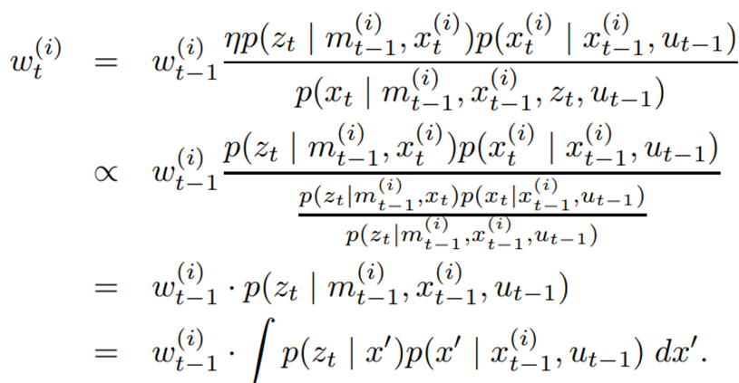

결국, 가중치는 $p(z_{t}|x)$로 표현되는 현재 pose에서의 scan 확률과 robot의 pose의 확률에 비례하게 됩니다. 즉, Scan값에서 유의미한 영역일수록 높은 가중치를 가진다는 얘기라고 할 수 있습니다.

2. Adaptive Resampling

낮은 가중치를 가지고 있는 파티클들은 높은 가중치의 파티클에게 대체되고는 합니다. Resampling step은 좋은 samples을 제거할 수 있으며, 이는 paricle impoverishment문제로 귀결됩니다. 따라서 언제 resampling을 진행할 지에 대한 명확한 기준이 필요합니다.

$N_{eff}$는 paricle set이 target posterir를 얼마나 잘 표현하는지 평가하는 샘플 크기입니다. 만약, 샘플이 target distribution으로 부터 나왔다면, 모든 파티클들의 중요도는 갖게 됩니다. Target distribution의 근사가 잘못될 수록, importance의 variance는 더욱 커진다고 할 수 있습니다.

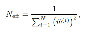
만약 $N_{eff}$가 threshold(N/2)보다 작으면, resampling을 진행하게 됩니다. 이렇게 하면, replacing의 횟수가 줄어들고 필요시에만 replacing이 되는 효과가 있습니다.

gMapping 단계별 알고리즘

먼저 gMapping의 pseudo code는 아래와 같습니다.

1) 모든 파티클에 대해서, odometry 모델을 이용하여 현재 pose를 추정합니다.

2) 이전상태까지의 map과 현재 포즈를 기반으로 Scan-Matching을 진행하여 최적의 포즈($x_{t}^i)$ 주변을 제한하게 됩니다. 만약 Scan-Matching이 실패하면, 기존의 motion model을 이용하여 포즈와 가중치를 계산하게 됩니다.

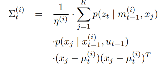
3) Scan-Matching의 local maximuim point($x_{t}^i)$ 중심으로 K개를 샘플링합니다

4) K sample의 mean과 covariance matrix를 계산합니다. 가중치 역시 계산합니다

5) 위에서 얻어낸 Gaussian approximation(proposal distribution)을 기반으로 새로운 포즈들을 샘플링하게 됩니다

6) Importance weight을 update합니다

7) 이전의 map($m_{1:t-1}^i)$과 현재의 포즈, 관찰값을 기반으로 새로운 map($m_{t}^i$)을 추정합니다.

8) $N_{eff}$에 따라 Resampling을 진행합니다.