HDF5
HDF는 계층적 데이터 형식(Hierarchical Data Format)을 뜻한다.
용량이 큰 데이터에 효율적으로 접근하기 위한 데이터 형식이다.
- HDF 데이터로 묶어내는 예제 코드
import h5py
import zipfile
import imageio
import os

%%time

# location of the HDF5 package, yours may be under /gan/ not /myo_gan/
hdf5_file = 'mount/My Drive/Colab Notebooks/myo_gan/celeba_dataset/celeba_aligned_small.h5py'

# how many of the 202,599 images to extract and package into HDF5
total_images = 20000

with h5py.File(hdf5_file, 'w') as hf:

    count = 0

    with zipfile.ZipFile('celeba/img_align_celeba.zip', 'r') as zf:
      for i in zf.namelist():
        if (i[-4:] == '.jpg'):
          # extract image
          ofile = zf.extract(i)
          img = imageio.imread(ofile)
          os.remove(ofile)

          # add image data to HDF5 file with new name
          hf.create_dataset('img_align_celeba/'+str(count)+'.jpg', data=img, compression="gzip", compression_opts=9)

          count = count + 1
          if (count%1000 == 0):
            print("images done .. ", count)
            pass

          # stop when total_images reached
          if (count == total_images):
            break
          pass

        pass
      pass
with h5py.File('celeba_aligned_small.h5py') as file_object:

    for group in file_object:
        print(group)
h5py 라이브러리를 이용하여 데이터셋에 접근할 수 있다.

또한 이 데이터셋은 딕셔너리에 접근하는 방식으로 접근한다.
import numpy as np
import matplotlib.pyplot as plt
with h5py.File('celeba_aligned_small.h5py') as file_object:
    dataset = file_object['img_align_celeba']
    image = np.array(dataset['7.jpg'])
    plt.imshow(image, interpolation='none')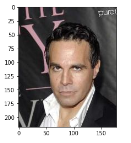
image.shape
3채널(rgb) 풀컬러 이미지이다.
data loader
from torch.utils.data import Dataset

class CelebADataset(Dataset):

    def __init__(self, file):
        self.file_object = h5py.File(file, 'r')
        self.dataset = self.file_object['img_align_celeba']

    def __len__(self):
        return len(self.dataset)

    def __getitem__(self, index):
        if (index >= len(self.dataset)):
            raise IndexError()
        img = np.array(self.dataset[str(index)+'.jpg'])
        return torch.cuda.FloatTensor(img) / 255.0

    def plot_image(self, index):
        plt.imshow(np.array(self.dataset[str(index)+'.jpg']), interpolation='nearest')
판별기
# discriminator class
import torch.nn as nn

class View(nn.Module):
    def __init__(self, shape):
        super().__init__()
        self.shape = shape,

    def forward(self, x):
        return x.view(*self.shape)

class Discriminator(nn.Module):

    def __init__(self):
        # initialise parent pytorch class
        super().__init__()

        # define neural network layers
        self.model = nn.Sequential(
            View(218*178*3),
            nn.Linear(3*218*178, 100),
            nn.LeakyReLU(),
            nn.LayerNorm(100),
            nn.Linear(100, 1),
            nn.Sigmoid()
        )

        # create loss function
        self.loss_function = nn.BCELoss()

        # create optimiser, simple stochastic gradient descent
        self.optimiser = torch.optim.Adam(self.parameters(), lr=0.0001)

        # counter and accumulator for progress
        self.counter = 0;
        self.progress = []

    def forward(self, inputs):
        # simply run model
        return self.model(inputs)

    def train(self, inputs, targets):
        # calculate the output of the network
        outputs = self.forward(inputs)

        # calculate loss
        loss = self.loss_function(outputs, targets)

        # increase counter and accumulate error every 10
        self.counter += 1;
        if (self.counter % 10 == 0):
            self.progress.append(loss.item())
        if (self.counter % 10000 == 0):
            print("counter = ", self.counter)

        # zero gradients, perform a backward pass, update weights
        self.optimiser.zero_grad()
        loss.backward()
        self.optimiser.step()

    def plot_progress(self):
        df = pd.DataFrame(self.progress, columns=['loss'])
        df.plot(ylim=(0), figsize=(16,8), alpha=0.1, marker='.', grid=True, yticks=(0, 0.25, 0.5, 1.0, 5.0))
해당 데이터셋은 218*178 사이즈의 rgb 이미지로 이루어져있다.
입력값 차원에서는 이 이미지를 평탄화해야되는데,
즉 218 x 178 x 3, 116,412 개의 입력을 받아야 한다.
평탄화 하는 함수는 pytorch에서 모듈화되어있지 않은데,
다음과 같은 코드를 사용하면 된다.
class View(nn.Module):
	def __init__(self, shape):
    	super().__init__()
    	self.shape = shape,

   def forward(self, x):
   return x.view(*self.shape)
View class를 통해 판별기 모델 안에서 평탄화를 진행할 수 있다.
mnist 예제처럼 random한 이미지 및 시드값을 만들어낼 수 있도록 준비하고
def generate_random_image(size):
    random_data = torch.rand(size)
    return random_data

def generate_random_seed(size):
    random_data = torch.randn(size)
    return random_data
%%time
import torch
D = Discriminator()
D.to(device)
if torch.cuda.is_available():
torch.set_default_tensor_type(torch.cuda.FloatTensor)
device = torch.device("cuda" if torch.cuda.is_available() else "cpu")
for image_data_tensor in celeba_dataset:
D.train(image_data_tensor, torch.cuda.FloatTensor([1.0]))
D.train(generate_random_image((218,178,3)), torch.cuda.FloatTensor([0.0]))판별기가 진짜와 가짜를 식별할 수 있는지 확인해본다
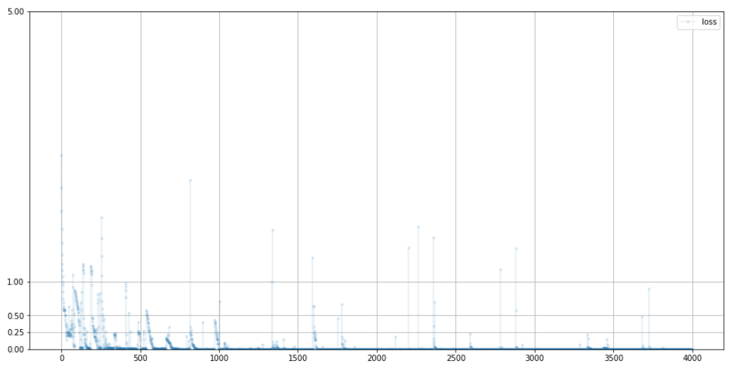
학습에 따른 loss를 보면 진짜 이미지 식별은 가능하다
생성기
# generator class

class Generator(nn.Module):

    def __init__(self):
        # initialise parent pytorch class
        super().__init__()

        # define neural network layers
        self.model = nn.Sequential(
            nn.Linear(100, 3*10*10),
            nn.LeakyReLU(),
            nn.LayerNorm(3*10*10),

            nn.Linear(3*10*10, 3*218*178),
            nn.Sigmoid(),
            View((218,178,3))
        )

        # create optimiser, simple stochastic gradient descent
        self.optimiser = torch.optim.Adam(self.parameters(), lr=0.0001)

        # counter and accumulator for progress
        self.counter = 0;
        self.progress = []

    def forward(self, inputs):
        # simply run model
        return self.model(inputs)

    def train(self, D, inputs, targets):
        # calculate the output of the network
        g_output = self.forward(inputs)

        # pass onto Discriminator
        d_output = D.forward(g_output)

        # calculate error
        loss = D.loss_function(d_output, targets)

        # increase counter and accumulate error every 10
        self.counter += 1;
        if (self.counter % 10 == 0):
            self.progress.append(loss.item())

        # zero gradients, perform a backward pass, update weights
        self.optimiser.zero_grad()
        loss.backward()
        self.optimiser.step()

    def plot_progress(self):
        df = pd.DataFrame(self.progress, columns=['loss'])
        df.plot(ylim=(0), figsize=(16,8), alpha=0.1, marker='.', grid=True, yticks=(0, 0.25, 0.5, 1.0, 5.0))
판별기와 반대로 입력 -> 출력 개수를 조절하고
View 클래스를 이용하여 평탄화된 값들을 다시 3차원 텐서로 변경한다
- 생성기 확인
G = Generator()
G.to(device)

output = G.forward(generate_random_seed(100))
img = output.detach().cpu().numpy()
plt.imshow(img, interpolation='none', cmap='Blues')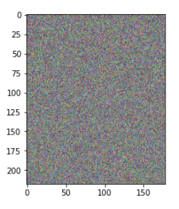
임의의 이미지를 생성 가능한 모습
훈련하기
D = Discriminator()
D.to(device)
G = Generator()
G.to(device)
epochs = 1
for epoch in range(epochs):
print("epoch = ", epoch + 1)
for image_data_tensor in celeba_dataset:
# 1단계, 참에 대한 판별기 훈련
D.train(image_data_tensor, torch.cuda.FloatTensor([1.0]))
# 2단계, 거짓에 대한 판별기 훈련
D.train(G.forward(generate_random_seed(100)).detach(), torch.cuda.FloatTensor([0.0]))
# 3단계, 생성기 훈련
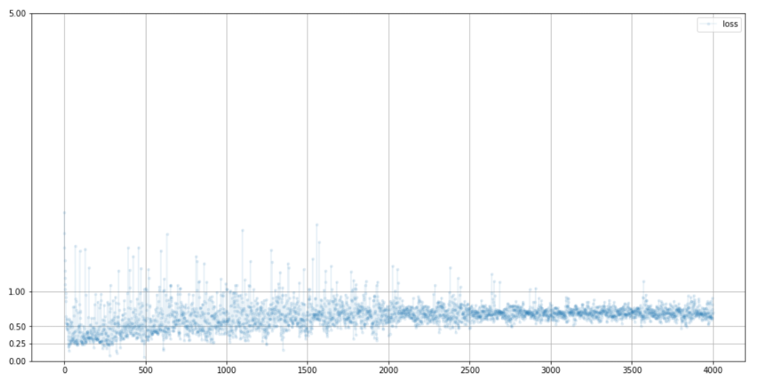
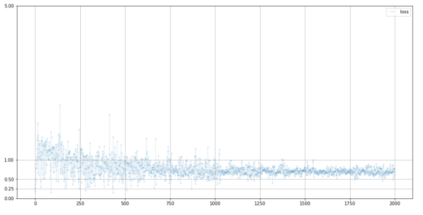
G.train(D, generate_random_seed(100), torch.cuda.FloatTensor([1.0]))- 훈련과정 loss 분석
loss가 bce의 이상적인 값인 0.69에 수렴하고 있는 모습
즉, 생성기와 판별기의 밸런스가 이상적인 상태다
-
판별기
-
생성기
- 생성되는 이미지 확인
f, axarr = plt.subplots(2,3, figsize=(16, 8))
for i in range(2):
    for j in range(3):
        output = G.forward(generate_random_seed(100))
        img = output.detach().cpu().numpy()
        axarr[i, j].imshow(img, interpolation='none', cmap='Blues')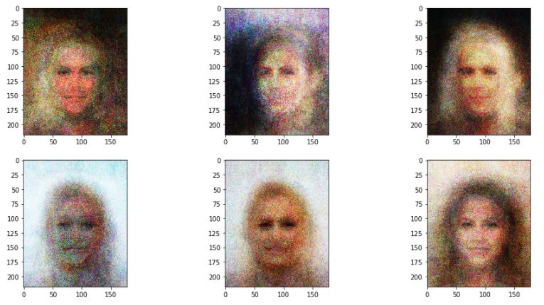
- epochs를 6까지 늘렸을 때의 모습(41분 소요)
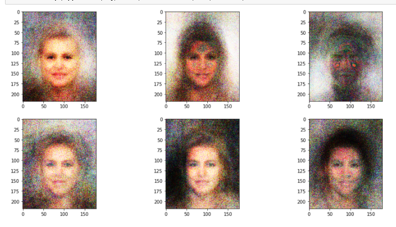
조금 더 선명해진 모습

오래 공부하는 사람