선형대수 : 03 선형대수학 - 4 : 역행렬, 역행렬 특징

yeppi1802·2024년 6월 30일
0

❇️ 요약

  • 역행렬이 존재하는 행렬 : Invertible Matrix
  • 2 × 2 행렬에서의 결정자 (ad - bc) : Determinant
  • 기본 행렬 : Elementary matrix
  • A1A^{-1}를 찾는 알고리즘 : Algorithm for Finding A1\textcolor{red}{A^{-1}}

📖 역행렬

🔆 역행렬

  • 역행렬이 존재하는 행렬 : Invertible Matrix
  • 2 × 2 행렬에서의 결정자 (ad - bc) : Determinant
  • 기본 행렬 : Elementary matrix
  • A1A^{-1}를 찾는 알고리즘 : Algorithm for Finding A1\textcolor{red}{A^{-1}}

🔆 1. 숫자의 승수 역수 - Multiplicative Inverse of a Number

  • 5의 역수는 15\frac 1 5
515=1    and    551=15^{-1}\cdot5=1 \;\;\text{and}\;\; 5\cdot5^{-1}=1

🔆 2. 역행렬이 존재하는 행렬 - Invertible Matrix

중요 핵심

CA=I    and    AC=ICA=I\;\;\text{and}\;\;AC=I
An  n×n  matrix  A  is said to be  invertible  if there is an  n×nmatrix  C  such thatCA=I    and    AC=I\text{An}\;n\times n \;\text{matrix}\;A\; \text{is said to be} \; \bold{invertible} \;\text{if there is an}\; n\times n \text{matrix}\;C\;\text{such that}\\ CA=I \;\;\text{and}\;\;AC=I
  • Invertible의 첫 번째 조건은 Row와 Column의 size가 동일해야함
  • AC=IAC = ICC 행렬이 있어야 하며 CC는 유일(unique) 해야 함
    • II는 단위 행렬
  • CC 대신 A1A^{-1}로 표기함
  • Matrix가
    • not invertible이면 singular matrix(해가 존재하지 않는 행렬)임
    • invertible이면 nonsingular matrix(해가 존재)함
A1A=I    and    AA1=IA^{-1}A = I \;\;\text{and}\;\; AA^{-1}=I

🔆 3. 이론 4 - Theorem 4

중요 핵심

If  adbc0,    A1=1adbc[dbca]\text{If}\;ad-bc\not =0,\;\;A^{-1}=\frac 1 {ad-bc} \begin{bmatrix} d & -b \\ -c & a \end{bmatrix}
Let A=[abcd]If  adbc0, then A is invertible and     A1=1adbc[dbca]If adbc=0, then A is not invertible.\begin{aligned} \text{Let }A = \begin{bmatrix} a & b \\ c & d \end{bmatrix}& \\\text{If}\;ad-bc\not =0,\text{ then }A\text{ is invertible and }\;\;& A^{-1}=\frac 1 {ad-bc} \begin{bmatrix} d & -b \\ -c & a \end{bmatrix} \\ \text{If } ad-bc =0,\text{ then }A\text{ is not invertible.}& \end{aligned}
  • A가 2×2 행렬일 때
    • adbc0ad-bc ≠ 0 이면 A는 invertrible
    • adbc=0ad-bc = 0 이면 not invertible
  • adbcad-bcpivot position이 2개 있을 조건을 의미하며 determinant(결정자)라고 부름
  • 어떤 matrix가 invertible을 판단할 때 determinant가 0인지 아닌지 확인하면 됨
A=[3456]A=\begin{bmatrix} 3 & 4 \\ 5 & 6 \end{bmatrix}
A1=12[6453]=[6/(2)4/(2)5/(2)3/(2)]=[325/23/2]A^{-1}= \frac 1 {-2} \begin{bmatrix} 6 & -4 \\ -5 & 3 \end{bmatrix} =\begin{bmatrix} 6/(-2) & -4/(-2) \\ -5/(-2) & 3/(-2) \end{bmatrix} =\begin{bmatrix} -3 & 2 \\ 5/2 & -3/2 \end{bmatrix}

🔆 4. 이론 5 - Theorem 5

중요 핵심

Au=b,A1Au=A1b,Iu=A1b,u=A1bA\bold{u}=\bold{b},\\ A^{-1}A\bold{u}=A^{-1}\bold{b}, \quad I\bold{u}=A^{-1}\bold{b}, \quad \bold{u}=A^{-1}\bold{b}
If A is an invertible n×n matrix, then for each b in Rn, the equation Ax=b has the unique solution x=A1b\text{If }A\text{ is an invertible }n\times n\text{ matrix, then for each } \bold{b} \text{ in } \Bbb{R^n},\\ \text{ the equation }A\bold{x}=\bold{b} \text{ has the unique solution }\bold{x}=A^{-1}\bold{b}
  • A가 invertible [n × n] matrix이면
    Rn\Bbb{R^n}공간에 있는 b에 대한 방정식 Ax=bA\text{x}=b유일한 해(x=A1b\text{x}=A^{-1}b)를 가짐

  • A의 inverse를 이용하면 쉽게 solution을 구할 수 있음

  • 증명

Au=b,A1Au=A1b,Iu=A1b,u=A1bA\bold{u}=\bold{b},\\ A^{-1}A\bold{u}=A^{-1}\bold{b}, \quad I\bold{u}=A^{-1}\bold{b}, \quad \bold{u}=A^{-1}\bold{b}
  • 예시
3x1+4x2=35x1+6x2=73x_1+4x_2=3\\ 5x_1+6x_2=7
x=A1b=[325/23/2][37]=[53]\bold{x}=A^{-1}\bold{b}= \begin{bmatrix} -3 & 2 \\ 5/2 & -3/2 \end{bmatrix} \begin{bmatrix} 3 \\ 7 \end{bmatrix}= \begin{bmatrix} 5 \\ -3 \end{bmatrix}

🔆 5. 이론 6 - Theorem 6

중요 핵심

(A1)1=A(A^{-1})^{-1}=A
(AB)1=B1A1(AB)^{-1}=B^{-1}A^{-1}
(AT)1=(A1)T(A^{T})^{-1}=(A^{-1})^{T}
  • AA가 invertible matrix이면 A1A^{-1}도 invertible임
a. If A is an invertible matrix, then A1 is invertible and (A1)1=A\text{a. If }A\text{ is an invertible matrix, then }A^{-1}\text{ is invertible and }\\\color{red}(A^{-1})^{-1}=A
  • (AB)1(AB)^{-1}B1A1B^{-1}A^{-1} 와 동일
  • ❗주의할 점 : 순서가 뒤바뀌어 B가 먼저 나온다는 것
b. If A and B are n×n invertible matrices, then so is AB,and the inverse of AB is the product of the inverses of A and B in the reverse order. That is, (AB)1=B1A1\text{b. If }A\text{ and }B\text{ are }n\times n\text{ invertible matrices, then so is }AB, \\\text{and the inverse of }AB\text{ is the product of the inverses of } A\text{ and }B\text{ in the reverse order.}\\ \text{ That is, }\\ \color{red} (AB)^{-1}=B^{-1}A^{-1}
  • AA가 invertible matrix이면 ATA^T도 invertible
    • ATA^T : 대각 행렬을 중심으로 돌린 행렬
c. If A is an invertible matrix, then so is AT, and the inverse of AT is the transpose of A1.That is,(AT)1=(A1)T\text{c. If }A\text{ is an invertible matrix, then so is }A^{T},\\ \text{ and the inverse of }A^T\text{ is the transpose of } A^{-1}.\\ \text{That is,}\\ \color{red} (A^{T})^{-1}=(A^{-1})^{T}

🔆 6. 기본 행렬 - Elementary Matrices

[참고 - 선형대수 : 03 선형대수학 - 2 : 소거법(elimination) 중 소거법]

  • 가우스 소거법에서 행할 수 있는 기본 행 연산(elementary row operations)
    1. 0이 아닌 상수를 행에 곱할 수 있다. (scaling)
    2. 두 행을 교환할 수 있다. (interchange)
    3. 한 행을 상수배 하여 다른 행에 더할 수 있다. (replacement)
  • 기본 행렬(elementary matrix)는 항등 행렬(identity matrix)에 단일 기본 행 연산(row operation)을 적용해서 얻어짐
Repalcement 적용한 행렬Interchange 적용한 행렬Scaling 적용한 행렬E1=[100010401],E2=[010100001],E3=[100010005]\begin{matrix} \text{Repalcement 적용한 행렬}& \text{Interchange 적용한 행렬}& \text{Scaling 적용한 행렬}\\ E_1=\begin{bmatrix} 1&0&0\\ 0&1&0\\ -4&0&1 \end{bmatrix}, & E_2=\begin{bmatrix} 0&1&0\\ 1&0&0\\ 0&0&1 \end{bmatrix}, & E_3=\begin{bmatrix} 1&0&0\\ 0&1&0\\ 0&0&5 \end{bmatrix} \end{matrix}
A=[abcdefghi]A=\begin{bmatrix} a&b&c\\ d&e&f\\ g&h&i \end{bmatrix}
  • E1E_1Replacement를 적용한 행렬
  • E1AE_1AAAReplacement를 적용한 것과 동일한 값 나옴
E1A=[100010401][abcdefghi]=[abcdefg4ah4bi4c]E_1A= \begin{bmatrix} 1&0&0\\ 0&1&0\\ -4&0&1 \end{bmatrix} \begin{bmatrix} a&b&c\\ d&e&f\\ g&h&i \end{bmatrix} =\begin{bmatrix} a&b&c\\ d&e&f\\ g-4a&h-4b&i-4c \end{bmatrix}
  • E2E_2Interchange를 적용한 행렬
  • E3E_3Scaling을 적용한 행렬
  • AA와 곱하면 AA에도 행 연산을 적용한 결과가 나옴
E2A=[010100001][abcdefghi]=[defabcghi]E_2A=\begin{bmatrix} 0&1&0\\ 1&0&0\\ 0&0&1 \end{bmatrix} \begin{bmatrix} a&b&c\\ d&e&f\\ g&h&i \end{bmatrix} =\begin{bmatrix} d&e&f\\ a&b&c\\ g&h&i \end{bmatrix}
E3A=[100010005][abcdefghi]=[abcdef5g5h5i]E_3A=\begin{bmatrix} 1&0&0\\ 0&1&0\\ 0&0&5 \end{bmatrix} \begin{bmatrix} a&b&c\\ d&e&f\\ g&h&i \end{bmatrix} =\begin{bmatrix} a&b&c\\ d&e&f\\ 5g&5h&5i \end{bmatrix}
  • 알 수 있는 특성
    • [m × n] matrix에 elementary row operation을 수행했다는 것
      어떤 [m × m] elementary matrix가 존재한다는 의미

    • A에 적용한 row operation을 [m × m] indentity matrix에 적용하면 EE가 생성

      If an elementary row operation is performed on an m×n matrix A, the resulting matrix can be written as EA, where the m×m metrix E is created by performing the same row operation on Im.\text{If an elementary row operation is performed on an }m\times n \text{ matrix }A,\\ \text{ the resulting matrix can be written as }EA,\\\text{ where the }m\times m\text{ metrix }E\text{ is created by performing the same row operation on }I_m.
    • elementary matrix EE가 invertible이면 EE의 inverse(역행렬)는 EEII로 변환하는 elementary matrix(기본 행렬) 임

      Each elementary matrix E is invertible.The inverse of E is the elementary matrix of the same typethat transforms E back into I.\text{Each elementary matrix }E\text{ is invertible.}\\ \text{The inverse of }E\text{ is the elementary matrix of the same type} \\ \text{that transforms }E\text{ back into }I.
      E1=[100010401],E11=[100010+401]E_1=\begin{bmatrix} 1&0&0\\ 0&1&0\\ -4&0&1 \end{bmatrix}, \quad E_1^{-1}=\begin{bmatrix} 1&0&0\\ 0&1&0\\ +4&0&1 \end{bmatrix}
      E1E11=[100010401][100010+401]=[100010001]=IE_1E_1^{-1}=\begin{bmatrix} 1&0&0\\ 0&1&0\\ -4&0&1 \end{bmatrix} \begin{bmatrix} 1&0&0\\ 0&1&0\\ +4&0&1 \end{bmatrix}= \begin{bmatrix} 1&0&0\\ 0&1&0\\ 0&0&1 \end{bmatrix}=I

🔆 7. 이론 7 - Theorem 7

An n×n matrix A is invertible if and only if A is row equivalent to In,and in this case, any sequence of elementary row operations that reduces A to In also transforms In into A1\text{An }n \times n \text{ matrix }A\text{ is invertible if and only if }A\text{ is row equivalent to }I_n,\\ \text{and in this case, any sequence of elementary row operations} \\ \text{ that reduces }A\text{ to }I_n \text{ also transforms }I_n \text{ into }A^{-1}
  • AA가 [n × n] invertible 행렬이면 AAInI_n과 행 상등(row equivalent)
  • AAInI_n으로 감소시키는 행 연산(row operation)은 InI_nA1A^{-1}로 변환
AE1AE2(E1A)Ep(Ep1E1A)=InA \sim E_1A \sim E_2(E_1A)\sim \cdots \sim E_p(E_{p-1}\cdots E_1A) = I_n
EpE1A=InE_p\cdots E_1A = I_n
(EpE1)1(EpE1)A=(EpE1)1InA=(EpE1)1\begin{aligned} (E_p\cdots E_1)^{-1}(E_p\cdots E_1)A &= (E_p\cdots E_1)^{-1}I_n\\ A&=(E_p\cdots E_1)^{-1} \end{aligned}
A1=[(EpE1)1]=EpE1A^{-1}=[(E_p\cdots E_1)^{-1}]=E_p\cdots E_1

🔆 8. A1A^{-1}를 찾는 알고리즘 - Algorithm for Finding A1A^{-1}

  • AA가 [m × n]이고 invertible이면 항등 행렬(identity matrix)를 이용해서 A1A^{-1}를 찾을 수 있음
ALGORITHM FOR FINDING A1Row reduce the augmented matrix [AI].If A is row equivalent to I, then [AI] is row equivalent to [IA1].A does not have an inverse.\textcolor{blue}{\textsf{ALGORITHM FOR FINDING }A^{-1}}\\ \text{Row reduce the augmented matrix }[A\quad I].\\ \text{If }A\text{ is row equivalent to }I,\text{ then }[A\quad I] \text{ is row equivalent to }[I\quad A^{-1}].\\ A \text{ does not have an inverse.}
  • 예시
A=[012103438]A=\begin{bmatrix} 0&1&2\\ 1&0&3\\ 4&-3&8 \end{bmatrix}
Interchange[AI]=[012103438A100010001I][103010012100438001]    ReplacementReplacement    (1×4,1+3=new3)(2×3,2+3=new3)[103010012100034041][103010012100002341]Scaling(3÷2)[1030100121000013/221/2]    Replacement    (3×3,3+1=new1)(3×2,3+2=new2)[100010001I9/273/22413/221/2A1]=[IA1]\begin{aligned} &\qquad\qquad\qquad\qquad\qquad\qquad\qquad\qquad\quad Interchange \\ [A\quad I]&= \begin{bmatrix} \boxed{ \begin{matrix} 0&1&2\\ 1&0&3\\ 4&-3&8 \end{matrix}}^A& \boxed{ \begin{matrix} 1&0&0\\ 0&1&0\\ 0&0&1 \end{matrix}}^I \end{bmatrix} \sim \begin{bmatrix} \textcolor{red}1&\textcolor{red}0&\textcolor{red}3&\textcolor{red}0&\textcolor{red}1&\textcolor{red}0\\ \textcolor{red}0&\textcolor{red}1&\textcolor{red}2&\textcolor{red}1&\textcolor{red}0&\textcolor{red}0\\ 4&-3&8&0&0&1 \end{bmatrix} \\\\ & \qquad\qquad\;\;Replacement\qquad\qquad \qquad Replacement \\&\;\;\quad\scriptsize (1행\times -4,\;\;1행 + 3행 =new 3행 )\qquad\scriptsize (2행\times 3,\;\;2행 + 3행 =new 3행 ) \\& \sim\begin{bmatrix} 1&0&3&0&1&0\\ 0&1&2&1&0&0\\ \textcolor{red}0&\textcolor{red}{-3}&\textcolor{red}{-4}&\textcolor{red}0&\textcolor{red}{-4}&\textcolor{red}1 \end{bmatrix}\sim \begin{bmatrix} 1&0&3&0&1&0\\ 0&1&2&1&0&0\\ \textcolor{red}0&\textcolor{red}0&\textcolor{red}2&\textcolor{red}3&\textcolor{red}{-4}&\textcolor{red}1 \end{bmatrix} \\\\& \qquad\qquad Scaling\scriptsize(3행 \div 2) \\& \sim\begin{bmatrix} 1&0&3&0&1&0\\ 0&1&2&1&0&0\\ \textcolor{red}0&\textcolor{red}0&\textcolor{red}1&\textcolor{red}{3/2}&\textcolor{red}{-2}&\textcolor{red}{1/2} \end{bmatrix} \\\\& \qquad\qquad\;\;Replacement \\&\;\;\quad \scriptsize (3행\times -3,\;\;3행 + 1행 =new 1행)\;\;\; (3행\times -2,\;\;3행 + 2행 =new 2행 ) \\& \sim\begin{bmatrix} &\boxed{ \begin{matrix} \textcolor{red}1&\textcolor{red}0&\textcolor{red}0\\ \textcolor{blue}0&\textcolor{blue}1&\textcolor{blue}0\\ 0&0&1\\ \end{matrix} }^I&\boxed{ \begin{matrix} \textcolor{red}{-9/2}&\textcolor{red}7&\textcolor{red}{-3/2}\\ \textcolor{blue}{-2}&\textcolor{blue}4&\textcolor{blue}{-1}\\ 3/2&-2&1/2 \end{matrix} }^{A^{-1}} \end{bmatrix}=[I\quad A^{-1}] \end{aligned}

이 방법은 4 × 4부터 굉장히 복잡하여 손으로 구하는건 거의 불가능


📖 역행렬의 특징

🔆 1. 이론 8. 역행렬 이론 - Theorem 8. The Invertible Matrix Theorem

  • AAinvertible이면 다음 조건을 다 만족하고, not invertible이면 다음 조건을 만족하지 않음
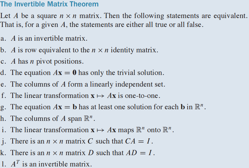
  • Ax=0A\text{x}=0은 trivial solution만을 갖으므로 independent, n pivot position을 만족
  • n개의 pivot position을 만족하므로 one-to-one도 성립
  • AA는 solution이 있으므로 AAR\Bbb{R}공간에 span하고, onto도 성립

🔆 2. 역선형 변환 - Invertible Linear Transformation

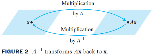
  • linear Transformation이 invertible이라고 불릴 조건은 다음과 같음
A linear transformation T:RnRn is said to be invertible if there exists a function S:RnRn such that(1)S(T(x))=xfor all x in Rn(2)T(S(x))=xfor all x in Rn\text{A linear transformation }T : \Bbb{R}^n \rarr \Bbb{R}^n \text{ is said to be }\bold{invertible}\\ \text{ if there exists a function }S:\Bbb{R}^n \rarr \Bbb{R}^n\text{ such that}\\ (1)\qquad S(T(\bold{x})) = \bold{x} \quad \text{for all }\bold{x} \text{ in }\Bbb{R}^n\\ (2)\qquad T(S(\bold{x})) = \bold{x} \quad \text{for all }\bold{x} \text{ in }\Bbb{R}^n
  • x의 image에 S 함수를 위하면 원래 x로 돌아옴
  • S 함수가 존재하는 경우에 T는 invertible하다고 함

🔆 3. 이론 9 - Theorem 9

  • 선형 변환(linear transformation)은 항상 표준 행렬(standard matrix)이 존재
  • T가 invertible이면 A(standard matrix)도 invertible 함
  • 또, 선형 변환(linear transformation) SS함수는S(x)=A1xS(\bold{x})=A^{-1}\bold{x}로 주어짐
Let T:RnRn be a linear transformation and let A be the standard matrix for T.Then T is invertible if and only if A is an invertible matrix.In that case, the linear transformation S given by S(x)=A1x is the unique function satisfying equations (1) and (2)\text{Let }T:\Bbb{R}^n \rarr \Bbb{R}^n\text{ be a linear transformation and let }A\text{ be the standard matrix for }T.\\ \text{Then }T\text{ is invertible if and only if }A\text{ is an invertible matrix.}\\ \text{In that case, the linear transformation }S\text{ given by }S(\bold{x})=A^{-1}\bold{x}\text{ is the unique function satisfying equations (1) and (2)}
profile
제로베이스 DA7 김예빈입니다.

0개의 댓글