지난 포스팅에서는 XGBoost 모델링 과정을 설명했습니다:) 이번에는 시계열 데이터나 텍스트와 같은 도메인에서 강력한 성능을 발휘하는 RNN(Recurrent Neural Network) 모델링 과정에 대해서 다뤄보겠습니다.

모델링: RNN (Recurrent Neural Network)

import pandas as pd
import numpy as np
from sklearn.model_selection import train_test_split
from tensorflow.keras.preprocessing.text import Tokenizer
from tensorflow.keras.preprocessing.sequence import pad_sequences
from tensorflow.keras.models import Sequential
from tensorflow.keras.layers import Embedding, LSTM, Dense, Dropout
from tensorflow.keras.callbacks import EarlyStopping, ReduceLROnPlateau
from sklearn.metrics import classification_report

data = pd.read_csv('/content/drive/MyDrive/spp_project/data_result.csv', index_col='type') #type열을 인덱스로 설정.

X = data['posts'] #설명변수
y = data.index #예측변수

# Train/test split
X_train, X_test, y_train, y_test = train_test_split(X_padded, y, test_size=0.2, random_state=42)

# numpy배열로 변환
X_train = np.array(X_train)
X_test = np.array(X_test)
y_train = np.array(y_train)
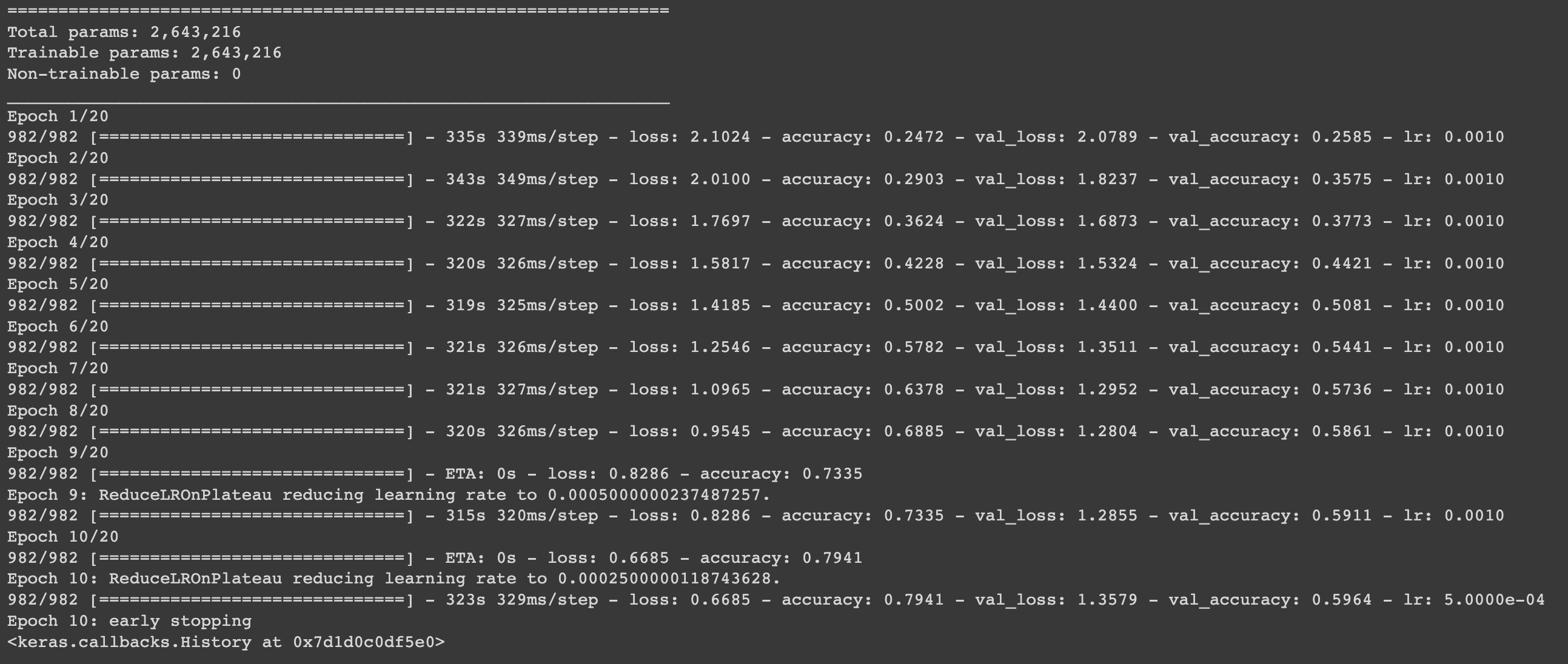
y_test = np.array(y_test)

모델링은 총 2가지로 학습을 진행했습니다. 2안은 lstm layer를 한 층 더 추가하고 drop out 비율을 늘렸습니다.

모델링 1안

# 모델 정의
model = Sequential()
model.add(Embedding(input_dim=max_words, output_dim=256, input_length=max_len))
model.add(LSTM(64, dropout=0.2))
model.add(Dense(len(label_to_int), activation='softmax'))  # Use len(label_to_int) as the number of units

# 모델 컴파일
model.compile(loss='sparse_categorical_crossentropy', optimizer='adam', metrics=['accuracy'])

model.summary()

# Early stopping callback 설정
early_stopping = EarlyStopping(monitor='val_loss', patience=2, verbose=1)

# Learning rate reduction callback 설정
reduce_lr = ReduceLROnPlateau(monitor='val_loss', factor=0.5, patience=1, verbose=1)

# 모델 학습
batch_size = 64
epochs = 20
model.fit(X_train, y_train_int, batch_size=batch_size, epochs=epochs,
          validation_split=0.2, callbacks=[early_stopping, reduce_lr])

early stopping: 검증 데이터(validation data)의 성능을 모니터링하여 학습을 조기중단 시키는 역할을 합니다. 성능이 개선되지 않을 때 학습을 중단하여 과적합을 방지하거나 학습 시간을 단축할 수 있습니다.

• monitor: 모니터링할 지표 ex) 'val_loss', 'val_accuracy'
• patience: 성능이 개선되지 않아도 몇 번까지 기다릴지 지정
• verbose: 출력 여부 ex) 0: 출력o, 1: 출력x
• resotre_best_weights: 최상의 모델 가중치로 복원할 지 여부

ReduceLROnPlateau: 학습률을 동적으로 조절하는 역할을 합니다. 검증 데이터(validation data)의 성능이 개선되지 않을 때, 학습률을 줄여서 모델이 더 나은 지점으로 수렴하도록 돕습니다.

• monitor: 모니터링할 지표
• factor: 학습률을 줄일 비율(새 학습률 = 현재 학습률*factor)
• verbose: 출력 여부
• min_lr: 학습률의 하한 값

아래의 결과를 보면, early stopping의 patience = 2로 설정했지 때문에 epoch 2개에서 연속으로 val_loss가 증가하면 성능이 개선되지 않는 것으로 학습이 조기 종료 되는 것을 확인할 수 있습니다.

# 예측
pred_probs = model.predict(X_test)
pred_classes = np.argmax(pred_probs, axis=1)

# classification report 계산 및 출력
report = classification_report(y_test_int, pred_classes, target_names=label_to_int.keys())
print(report)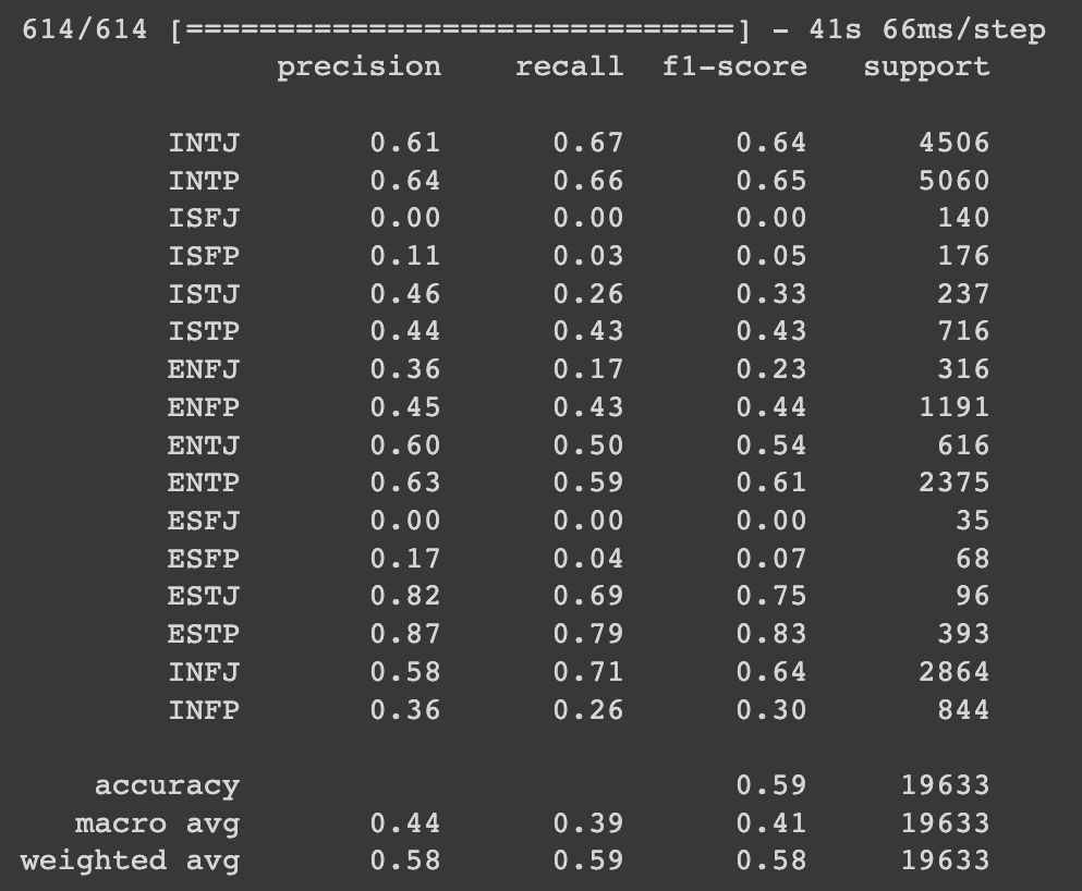

classification report를 보면, support(각 클래스에 속한 샘플의 수)가 적은 클래스는 대체적으로 precision, recall, f1-score가 모두 낮은 것을 볼 수 있습니다. 성능을 높이기 위해서는 파라미터 튜닝(모델의 layer 층 개수 조절 등), 클래스 불균형 해결, drop out 비율 조절 등의 방법이 있습니다.

처음으로 고려했던 방법은 가중치 조정을 통한 '클래스 불균형 해결'이었는데, 오히려 정확도가 심하게 낮아지고 검증 데이터에 대한 성능이 거의 개선되지 않고 학습이 조기 종료되어 다른 방법을 시도했습니다.

코드에는 사용하지 않았지만, 가중치 조정에 대해 궁금하신 분들은 참고 바랍니다.가중치 조정 방법은 다음과 같습니다.

 클래스 불균형 문제를 해결하기 위해서는 class_weight 매개변수를 사용하면 됩니다. 
 class_weight는 손실 함수 계산 시 각 클래스에 적용할 가중치를 지정하는 매개변수로, 
 불균형한 클래스에 높은 가중치를 부여하여 모델이 불균형한 데이터를 더 잘 학습할 수 있도록 도와줍니다.

# 필요한 모듈 임포트
from sklearn.utils.class_weight import compute_class_weight

# 클래스 가중치 계산
class_weights = compute_class_weight(class_weight = "balanced", classes = np.unique(y_train_int), y = y_train_int)
class_weight_dict = {i: w for i, w in enumerate(class_weights)}
.
.
(생략)
.
.
# 매개변수에 class_weight=class_weight_dict 추가
model.fit(X_train, y_train_int, batch_size=batch_size, epochs=epochs,
          validation_split=0.2, callbacks=[early_stopping, reduce_lr], class_weight=class_weight_dict)

모델링 2안

# Define the model
model = Sequential()
model.add(Embedding(input_dim=max_words, output_dim=256, input_length=max_len))
model.add(LSTM(128, dropout=0.3, return_sequences=True))
model.add(LSTM(128, dropout=0.3))
model.add(Dense(len(label_to_int), activation='softmax'))  # Use len(label_to_int) as the number of units

# Compile the model
model.compile(loss='sparse_categorical_crossentropy', optimizer='adam', metrics=['accuracy'])

# Print model summary
model.summary()

# Early stopping callback
early_stopping = EarlyStopping(monitor='val_loss', patience=2, verbose=1)

# Learning rate reduction callback
reduce_lr = ReduceLROnPlateau(monitor='val_loss', factor=0.5, patience=1, verbose=1)

# Train the model
batch_size = 64
epochs = 30
model.fit(X_train, y_train_int, batch_size=batch_size, epochs=epochs,
          validation_split=0.2, callbacks=[early_stopping, reduce_lr])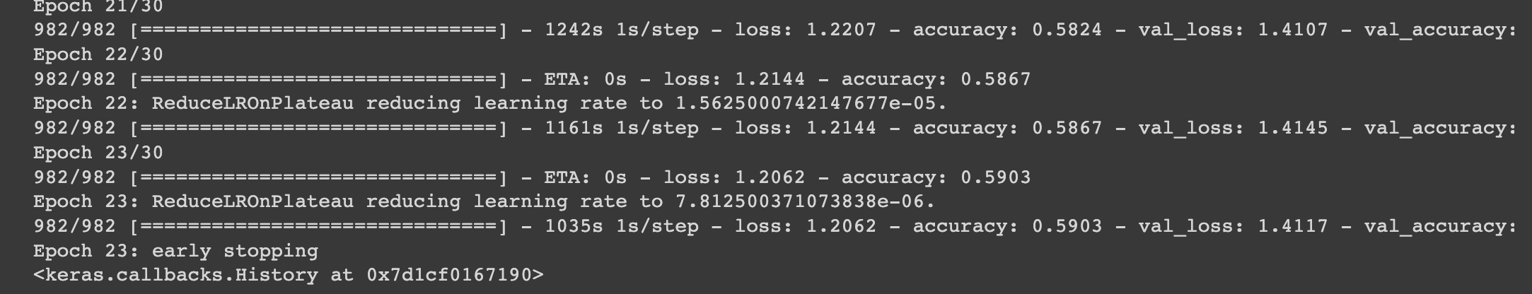

# Predict classes
pred_probs = model.predict(X_test)
pred_classes = np.argmax(pred_probs, axis=1)

# Calculate classification report
report = classification_report(y_test_int, pred_classes, target_names=label_to_int.keys())
print(report)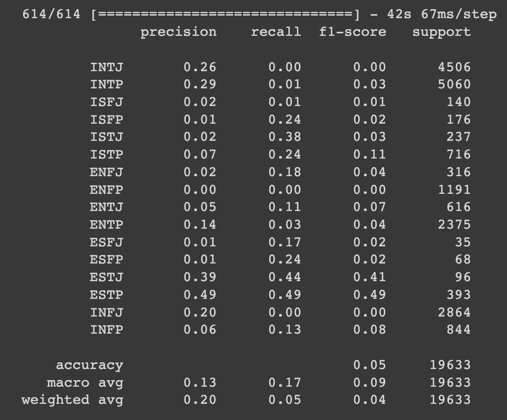

2안도 마찬가지로 support(각 클래스에 속한 샘플의 수)가 적은 클래스는 대체적으로 precision, recall, f1-score가 모두 낮은 것을 볼 수 있습니다. 클래스 불균형 해결이 가장 중요할 것 같다는 생각이 들었고, 가중치 조정으로 계속 시도를 해보았지만 해결이 안되었기 때문에 처음에 사용하던 LinearSVC 모델에 데이터 리샘플링을 추가해보기로 결정했습니다.

마치며..

딥러닝 모델링 경험이 많지 않아서 더욱 많은 시간을 투자했지만 좋은 결과는 얻지 못했던 것 같습니다. 이번에 딥러닝 모델링을 직접 해보면서 공부해야할 부분이 많다는 것을 느꼈습니다. 다양한 에러와 좋지 않은 성능을 마주하는 등 많은 시행착오를 겪으면서, 배울 수 있었고 부족함을 많이 느꼈습니다. 초반에 짰던 알고리즘부터 최종 결과물까지 비교를 하면 많이 성장한 것 같다는 생각도 들었습니다. 다음 포스팅에서는 처음 짰던 LinearSVC 코드와 최종 모델로 완성된 LinearSVC 코드에 대한 설명을 모두 작성하겠습니다.