
💡3.4. F1 스코어(F1 Score)
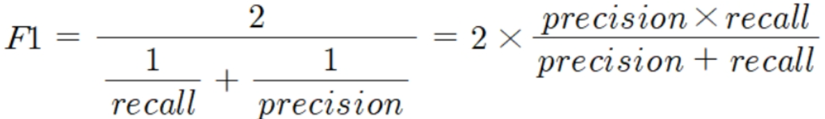
F1 스코어
- 정밀도와 재현율을 결합한 지표
- 정밀도와 재현율이 어느 한쪽으로 치우치지 않는 수치를 나타낼 때 상대적으로 높은 값을 가짐
- 사이킷런에서
f1_score()API 제공
from sklearn.metrics import f1_score

f1 = f1_score(y_test, pred)
print('F1 스코어 : {0:.4f}'.format(f1))
📈3.5. ROC 곡선과 AUC
ROC곡선
- ROC 곡선과 이에 기반한 AUC 스코어 : 이진 분류의 예측 성능 측정에서 중요 지표임
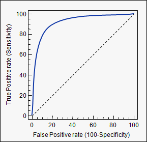
- ROC 곡선 (Receiver Operation Characteristic Curve) : 수신자 판단 곡선
- FPR(False Positive Rate)이 변할 때 TPR(True Positive Rate)이 어떻게 변하는지 나타냄
- X축=FPR, Y축=TPR
- 민감도(TPR) : 재현율
- TPR = TP/(FN+TP)
- 실제값 positive(양성)가 정확히 예측돼야 하는 수준
- 질병 있는 사람을 아프다고 양성판정
- 특이성(specificity, TNR) : 민감도
- TNR(True Negative Rate)=TN/(FP+TN)
- 실제값 negative(음성)가 정확히 예측돼야 하는 수준
- 건강한 사람을 건강하다고 음성 판정
- X축인
FPR = FP/(FP+TN) = 1 - TNR = 1 - 특이성
- 가운데 직선은 ROC 곡선의 최저값. 랜덤 수준의 이진 분류의 ROC 직선. AUC=0.5 -> 가운데 직선에 ROC 곡선이 가까울 수록 성능 떨어지는 것
- FPR을 0~1까지 변경하며 TPR의 변화값 구함
- FPR을 변경하는 방법 : 분류 결정 임곗값(positive 에측값을 결정하는 확률의 기준)을 변경하는 것
- FPR을 0으로 만들려면? 임곗값=1로 -> Positive 예측 기준이 매우 높아 분류기(classifier)가 임곗값보다 높은 확률 가진 데이터를 positive로 예측할 수 없음 -> FP=0 -> FPR=0
- FPR을 1으로 만들려면? 임곗값=0로 -> Negative 예측이 없음 -> TN=0 -> FPR=1
- FPR을 변경하는 방법 : 분류 결정 임곗값(positive 에측값을 결정하는 확률의 기준)을 변경하는 것
- 따라서 ROC 곡선은 임곗값을 1부터 0까지 거꾸로 변화시키며 구한 재현율 곡선의 형태와 비슷
사이킷런의 ROC 곡선
roc_curve()APIprecision_recall_curve()API와 사용법 유사 <-> 반환값 구성이 다름- 입력 파라미터
y_true= 실제 클래스값 array, 형상=[데이터 건수]y_score= predict_proba()의 반환값 배열에서 positive 칼럼의 에측 확률이 보통 사용됨, 형상=[n_smaples]
- 반환값
fpr= fpr을 배열로 반환tpr= tpr을 배열로 반환thresholds= threshold 배열
### 타이타닉 생존자 예측 데이터셋 이용
from sklearn.metrics import roc_curve

#레이블값이 1일 때의 예측 확률을 추출
pred_proba_class1 = lr_clf.predict_proba(x_test)[:, 1]

fprs, tprs, thresholds = roc_curve(y_test, pred_proba_class1)
#반환된 임곗값 배열에서 샘플로 데이터 추출하되, 임곗값을 5 step으로 추출
#thresholds[0]은 max(예측확률)+1로 임의 설정됨. 이를 제외하기 위해 np.arange를 1로 시작
thr_index = np.arange(1, thresholds.shape[0], 5)
print('샘플 추출을 위한 임곗값 배열의 index : ', thr_index)
print('샘플 index로 추출한 임곗값 : ', np.round(thresholds[thr_index], 2))

#5step 단위로 추출된 임곗값에 따른 FPR, TPR 값
print('샘플 임곗값 별 FPR : ', np.round(fprs[thr_index], 3))
print('샘플 임곗값 별 TPR : ', np.round(tprs[thr_index], 3))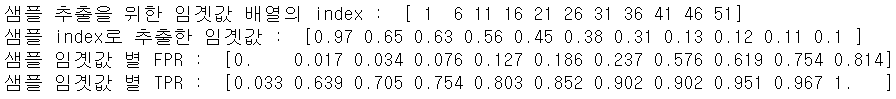
### ROC 곡선 시각화

import matplotlib.pyplot as plt

def roc_curve_plot(y_test, pred_proba_class1):
    fprs, tprs, thresholds = roc_curve(y_test, pred_proba_class1)
    plt.plot(fprs, tprs, label="ROC")
    plt.plot([0, 1], [0, 1], 'k--', label="Random")

    start, end = plt.xlim()
    plt.xticks(np.round(np.arange(start, end, 0.1), 2))
    plt.xlim(0, 1); plt.ylim(0, 1)
    plt.xlabel('FPR(1-Sensitivity)'); plt.ylabel('TPR(Recall)')
    plt.legend()

roc_curve_plot(y_test, pred_proba_class1).png)
AUC 스코어
- ROC와 AUC
- ROC 곡선 : FPR, TPR의 변화값을 보는 데 ㅣㅇ용
- AUC 값 : 분류 성능의 지표로 사용. ROC 곡선 면적에 기반
- AUC(Area Under Curve) : ROC 곡선의 밑 면적 구한 것. 1에 가까울수록 좋은 수치
- FPR이 작은 상태에서 얼마나 큰 TPR을 얻느냐가 AUC 수치 커지는 데 관건임
- 가운데 직선에서 멀어지고, 좌상단 모서리로 가파르게 곡선 이동살 후록 직사각형 가까운 곡선 되어 면적=1에 가까워짐
- 가운데 대각선 수준은 0.5이므로, 보통 분류는 0.5이상의 AUC 값 가짐
from sklearn.metrics import roc_auc_score

pred_proba = lr_clf.predict_proba(x_test)[:, 1]
roc_score = roc_auc_score(y_test, pred_proba)
print('ROC AUC 값 : {0:.4f}'.format(roc_score))
최종 get_clf_eval() 함수
from sklearn.metrics import accuracy_score, precision_score, recall_score, confusion_matrix

def get_clf_eval(y_test, pred=None, pred_proba=None):
    confusion = confusion_matrix(y_test, pred)
    accuracy = accuracy_score(y_test, pred)
    precision = precision_score(y_test, pred)
    recall = recall_score(y_test, pred)
    f1 = f1_score(y_test, pred)
    roc_auc = roc_auc_score(y_test, pred_proba)

    print('오차행렬 : ')
    print(confusion)

    print('정확도 : {0:.4f} , 정밀도 : {1:.4f} , 재현율 : {2:.4f} , F1 : {3:.4f}, AUC : {4:.4f}'.format(accuracy, precision, recall, f1, roc_auc))
🍦3.6. 피마 인디언 당뇨병 예측
피마 인디언 당뇨병 예측 데이터세트
- 당뇨병 여부 판단하는 머신러닝 예측 모델 수립하고 평가 지표 적용해보자
- 북아메리카 피마 지역 원주민의 2형 당뇨병 결과 데이터임
- 데이터 세트 피처
- Pregnancies = 임신 횟수
- Glucose = 포도당 부차 검사 수치
- BoolPressure = 혈압
- SkinThickness = 팔 삼두근 뒤쪽 피하지방 측정값
- Insulin = 혈청 인슐린
- BMI = 체질량지수
- DiabetesPedigreeFunction = 당뇨 내력 가중치 값
- Age = 나이
- Outcome = 클래스 결정값. 0 or 1
라이브러리 및 모듈 임포트
import numpy as np
import pandas as pd
import matplotlib.pyplot as plt
import matplotlib.ticker as ticker
%matplotlib inline

from sklearn.model_selection import train_test_split
from sklearn.metrics import accuracy_score, precision_score, recall_score, roc_auc_score, f1_score, confusion_matrix, precision_recall_curve, roc_curve
from sklearn.preprocessing import StandardScaler
from sklearn.linear_model import LogisticRegression
from sklearn.preprocessing import Binarizer
사용할 함수 사전제작
def get_clf_eval(y_test, pred=None, pred_proba=None):
    confusion = confusion_matrix(y_test, pred)
    accuracy = accuracy_score(y_test, pred)
    precision = precision_score(y_test, pred)
    recall = recall_score(y_test, pred)
    f1 = f1_score(y_test, pred)
    roc_auc = roc_auc_score(y_test, pred_proba)

    print('오차행렬 : ')
    print(confusion)

    print('정확도 : {0:.4f} , 정밀도 : {1:.4f} , 재현율 : {2:.4f} , F1 : {3:.4f}, AUC : {4:.4f}'.format(accuracy, precision, recall, f1, roc_auc))

def precision_recall_curve_plot(y_test, pred_proba_c1):
    #threshold ndarray와 이 threshold에 따른 정밀도, 재현율 ndarray 추출
    precisions, recalls, thresholds = precision_recall_curve(y_test, pred_proba_c1)
    #x축을 threshold값으로, y축을 정밀도, 재현율 값으로 각각 plot 수행. 정밀도는 점선
    plt.figure(figsize=(8, 6))
    threshold_boundary = thresholds.shape[0]
    plt.plot(thresholds, precisions[0:threshold_boundary], linestyle='--', label='precision')
    plt.plot(thresholds, recalls[0:threshold_boundary], label='recall')
    #threshold값 x축의 스케일을 0.1 단위로 변경
    start, end = plt.xlim()
    plt.xticks(np.round(np.arange(start, end, 0.1), 2))
    #각 축 라벨과 범례, 그리드 설정
    plt.xlabel("Threshold value")
    plt.ylabel("Precision and Recall Value")
    plt.legend()
    plt.grid()
    plt.show()

def get_eval_by_threshold(y_test, pred_proba_c1, thresholds):
    for custom_threshold in thresholds:
        binarizer = Binarizer(threshold=custom_threshold).fit(pred_proba_c1)
        custom_predict = binarizer.transform(pred_proba_c1)
        print("임곗값 : ", custom_threshold)
        get_clf_eval(y_test, custom_predict, pred_proba_c1)
데이터 로딩 및 사전 처리
#데이터 로딩 및 outcome 개수 확인
diabets_data = pd.read_csv('../kaggle/pima_indians_diabets/diabetes.csv')
print(diabets_data['Outcome'].value_counts())
diabets_data.head(3)

# 피처 타입과 null 개수 확인
diabets_data.info()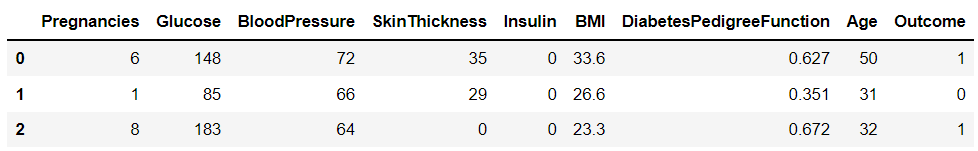
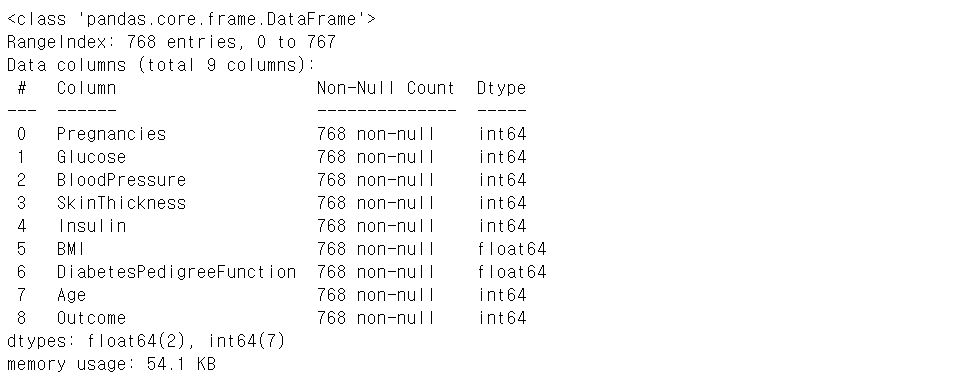
예측 모델 생성, 학습, 예측, 평가
x = diabets_data.iloc[:, :-1]
y = diabets_data.iloc[:, -1]
x_train, x_test, y_train, y_test = train_test_split(x, y, test_size=0.2, random_state=156, stratify=y)

lr_clf = LogisticRegression()
lr_clf.fit(x_train, y_train)
pred = lr_clf.predict(x_test)
pred_proba = lr_clf.predict_proba(x_test)[:, 1]

get_clf_eval(y_test, pred, pred_proba)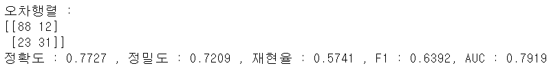
0값 대체하여 성능 개선하기
전체 데이터의 65프로가 Negative이므로 정확도보다 재현율에 초점 맞춰 변경해보자
- 먼저, 정밀도 재현율 곡선을 보고 임곗값 별 정밀도와 재현율 값의 변화 확인
- 아래 결과를 보면, 정밀도와 재현율이 0.42 정도면 균형 맞추나, 지표가 0.7이 안되게 낮음
pred_proba_c1 = lr_clf.predict_proba(x_test)[:, 1]
precision_recall_curve_plot(y_test, pred_proba_c1)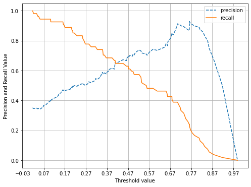
- 임계값을 인위적으로 조작하기 전에 값의 분포도부터 살펴보자
diabets_data.describe()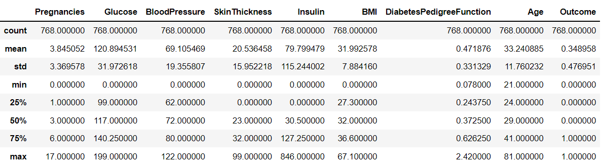
- min = 0인 경우가 많음 -> 0값의 건수 및 전체 데이터 건수 대비 몇 퍼센트 비율로 존재하는지 확인하자
#0값을 검사할 피처명 리스트
zero_features = ['Glucose', 'BloodPressure', 'SkinThickness', 'Insulin', 'BMI']

#전체 데이터 건수
total_count = diabets_data['Glucose'].count()

#피처별로 반복하면서 데이터값이 0인 데이터 건수를 추출하고, 퍼센트 계산
for feature in zero_features:
    zero_count = diabets_data[diabets_data[feature] == 0][feature].count()
    print('{0} 0 건수는 {1}, 퍼센트는 {2:.2f}%'.format(feature, zero_count, 100*zero_count/total_count))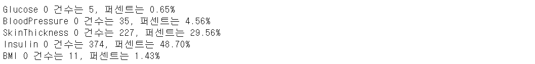
- 0값을 평균값으로 대체한 뒤, 다시 스케일링 및 학습~평가 수행
mean_zero_features = diabets_data[zero_features].mean()
diabets_data[zero_features] = diabets_data[zero_features].replace(0, mean_zero_features)

#변환값에 대해 피처 스케일링 적용해 변환
x = diabets_data.iloc[:, :-1]
y = diabets_data.iloc[:, -1]
scaler = StandardScaler()
x_scaled = scaler.fit_transform(x)
x_train, x_test, y_train, y_test = train_test_split(x_scaled, y, test_size=0.2, random_state=156, stratify=y)

lr_clf = LogisticRegression()
lr_clf.fit(x_train, y_train)
pred = lr_clf.predict(x_test)
pred_proba = lr_clf.predict_proba(x_test)[:, 1]

get_clf_eval(y_test, pred, pred_proba)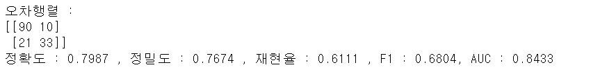
분류 결정 임곗값을 변화시켜 성능 개선
- 분류 결정 임곗값을 변화시키며 재현율 성능 수치 개선 확인
thresholds = [0.3, 0.33, 0.36, 0.39, 0.42, 0.45, 0.48, 0.50]
pred_proba = lr_clf.predict_proba(x_test)
get_eval_by_threshold(y_test, pred_proba[:, 1].reshape(-1, 1), thresholds)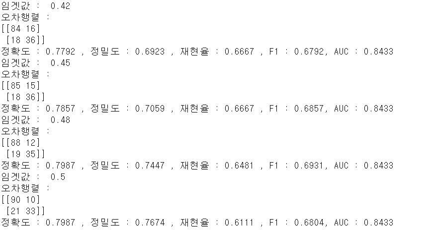
- 임곗값 0.48이 가장 좋아보임
binarizer = Binarizer(threshold=0.48)
pred_th_048 = binarizer.fit_transform(pred_proba[:, 1].reshape(-1, 1))
get_clf_eval(y_test, pred_th_048, pred_proba[:, 1])
🏫Inha Univ. Naval Architecture and Ocean Engineering & Computer Engineering (Undergraduate) / 🚢Autonomous Vehicles, 💡Machine Learning