
📚 Simple Linear Regression
저번 글에선 데이터 전처리를 하지 않고 Python 직접 구현 방식으로 Simple Linear Regression을 구현해 보았었다. 이번 글에서는 간략한 데이터 전처리를 진행한 후, Python, Tensorflow, sklearn으로 모델을 구현하여 각 모델의 차이를 확인해보자. 이번 글에서도 역시 Ozone Data Set을 이용할 것이다.
Data Loading
import numpy as np
import pandas as pd
df = pd.read_csv('/content/drive/MyDrive/KDT/data/ozone.csv') training_data = df[['Temp','Ozone']] print(df.shape) # (153, 6)
📚 Data Preprocessing
간단하게 결측치, 이상치를 처리하고 데이터 정규화까지 진행해보자.
이때 결측치 삭제 처리할 것이고, 이상치는 Z-Score를 사용하여 이상치를 찾아 마찬가지로 삭제 처리할 것이다. 데이터 정규화는 Min-Max Normalization을 사용할 것이다.
📚 결측치 처리
training_data = training_data.dropna(how='any')
display(training_data.shape) # (116, 2)
간단하게 pandas의 dropna 함수를 사용하여 결측치를 포함하고 있는 모든 행을 삭제한다.
📚 이상치 처리 (Z-Score)
from scipy import stats

zscore_threshold = 1.8 # zscore outliers 임계값 (2.0이하가 optimal)
이상치는 정규분포를 사용하는 Z-Score로 판별하여 삭제처리 할 것이다.
# Temp에 대한 이상치(지대점) 확인
outliers = training_data['Temp'][(np.abs(stats.zscore(training_data['Temp'])) > zscore_threshold)]
print(outliers)
# 7      59
# 14     58
# 17     57
# 20     59
# 119    97
# 121    96
# Name: Temp, dtype: int64

# Temp에 대한 이상치(지대점) 제거한 결과
training_data = training_data.loc[~training_data['Temp'].isin(outliers)]
print(training_data.shape)  # (110, 2)
우선, 독립변수인 Temp에 대해 지정한 zscore_threshold에 따라 지대점을 판별하고 마스크를 생성하여 이상치(지대점)를 삭제 처리한다.
# Ozone에 대한 이상치(Outlier) 확인
outliers = training_data['Ozone'][(np.abs(stats.zscore(training_data['Ozone'])) > zscore_threshold)]
print(outliers)
# 29     115.0
# 61     135.0
# 85     108.0
# 98     122.0
# 100    110.0
# 116    168.0
# 120    118.0
# Name: Ozone, dtype: float64

# Ozone에 대한 이상치 제거한 결과
training_data = training_data.loc[~training_data['Ozone'].isin(outliers)]
print(training_data.shape)  # (103, 2)
이후, 종속변수인 Ozone에 대하여도 지정한 zscore_threshold에 따라 지대점을 판별하고 마스크를 생성하여 이상치(Outlier)를 삭제 처리한다.
📚 정규화 처리 (Min-Max Normalization)
from sklearn.preprocessing import MinMaxScaler

scaler_x = MinMaxScaler()
scaler_t = MinMaxScaler()

scaler_x.fit(training_data['Temp'].values.reshape(-1,1))
scaler_t.fit(training_data['Ozone'].values.reshape(-1,1))

# Training Data Set

x_data = training_data['Temp'].values.reshape(-1,1)
t_data = training_data['Ozone'].values.reshape(-1,1)

x_data_norm = scaler_x.transform(x_data)
t_data_norm = scaler_y.transform(t_data)
여기서 모델이 각 변수들의 scale을 동일한 정도로 반영할 수 있도록 정규화를 진행한다. 이때, sklearn library를 사용하여 간단하게 Min-Max Normalization을 진행한다.
📚 Simple Linear Regression 구현 (Python)
이전 글에서 만들었던 코드를 그대로 사용하면 된다.
📚 Weight & bias 정의
W = np.random.rand(1, 1)
b = np.random.rand(1)
초기의 W, b 값은 랜덤으로 지정하고, 이를 회귀를 통해 데이터의 분포를 가장 잘 나타내는 직선을 그리는 값을 찾아가게 한다.
📚 loss function 정의
def loss_func(input_obj):

    input_W = input_obj[0].reshape(-1,1) # Weight를 matrix로 변환
    input_b = input_obj[1].reshape(-1,1)

    y = np.dot(x_data_norm,input_W) + input_b

    return np.mean(np.power((t_data_norm - y), 2))
우리는 loss 함수로 MSE를 사용할 것이기 때문에 MSE의 공식을 그대로 코드로 구현해 주었다.
📚 수치미분코드 정의
def numerical_derivative(f,x):

    # f : 미분하려고 하는 다변수 함수
    # x : 모든 변수를 포함하고 있는 numpy array(차원상관없음)

    delta_x = 1e-4
    derivative_x = np.zeros_like(x)  # 계산된 수치미분 값을 저장하기 위한 변수

    # iterator를 이용하여 입력변수 x에 대해 편미분 수행
    it = np.nditer(x, flags=['multi_index'])

    while not it.finished:

        idx = it.multi_index   # 현재의 index를 추출 => tuple형태로 리턴

        tmp = x[idx]
        x[idx] = tmp + delta_x
        fx_plus_delta = f(x)   # f(x + delta_x)

        x[idx] = tmp - delta_x
        fx_minus_delta = f(x)   # f(x - delta_x)

        derivative_x[idx] = (fx_plus_delta - fx_minus_delta) / (2 * delta_x)

        x[idx] = tmp

        it.iternext()

    return derivative_x
learning rate와 편미분을 통해 loss값이 최소가 되는 W와 b값을 update하기 위해 편미분을 코드로 구현한다.
📚 학습 진행
learning_rate = 1e-2

# 학습진행
for step in range(300000):

    input_param = np.concatenate((W.ravel(),b.ravel()),axis=0)

    derivative_result = learning_rate * numerical_derivative(loss_func, input_param)

    W = W - derivative_result[0].reshape(-1, 1)
    b = b - derivative_result[1].reshape(-1, 1)


    if step % 300000 == 0:
        print(f'W : {W}, b : {b}, loss : {loss_func(input_param)}')
        # 학습종료 후 W, b, loss value의 값
        W : [[0.79468511]], b : [-0.04818192], loss : 0.03032684147617442
loss 함수에 learning rate를 곱한 값을 이용하여 주어진 epochs 동안 W와 b를 경사하강법을 통해 update한다. 이를 통해 최종 W와 b 값을 구할 수 있고, 이를 이용하여 마지막에 그래프를 그려 다른 모델들과 비교해 볼것이다.
📚 예측
def predict(x):

    y = np.dot(x,W) + b

    return y

# 학습종료 후 예측 (화씨 62도일때 Ozone량)
# Min-Max Normalization을 이용했기 때문에 62 값을 그대로 이용하면 안된다.
predict_data = np.array([[62]])
predict_data_norm = scaler_x.transform(predict_data)
scaled_result = predict(predict_data_norm)
result = scaler_y.inverse_transform(scaled_result.reshape(-1,1))
print(result) # [[1.75864872]]
이제 학습이 완료되었다면, 예측을 할 차례이다. 이때 주의해야 할 것이 있는데, 정규화한 데이터에 대해 예측할 값을 입력할 때, 예측할 값도 정규화 처리를 해준 후 입력을 해야 올바른 값이 도출된다. 이때 도출된 예측 값 또한 정규화된 값으로 출력되기에, 예측 값에는 정규화 처리를 되돌려주는 작업이 필요하다.
📚 Simple Linear Regression 구현 (Tensorflow)
이번에는 Tensorflow의 keras를 통해 모델을 구현해보자.
📚 Model 생성
from tensorflow.keras.models import Sequential

keras_model = Sequential()
먼저 Sequential 모델을 사용하여 간단한 순차적인 구조를 가진 모델을 구현해보자.
📚 Layer 추가
from tensorflow.keras.layers import Flatten, Dense

input_layer = Flatten(input_shape=(1,))
output_layer = Dense(1, activation='linear')
먼저 입력층을 Flatten으로 현재 독립변수가 1개인 모델을 만들기 때문에 input_shape을 (1,)로 지정해준다. 이때 input_shape은 tuple을 사용하여 지정해주어야 한다. 또한 출력층으로는 Dense를 사용하는데, 출력값은 1개, activation에는 지금 선형 회귀 모델을 구현하고 있기 때문에 linear 함수로 지정해준다.
📚 Model 설정
from tensorflow.keras.optimizers import SGD

keras_model.compile(optimizer=SGD(learning_rate=1e-2), loss='mse')
이제 모델을 생성하고, 모델에 층을 만들어 주었다면, 이제 모델이 어떻게 학습을 진행할지 몇가지 설정을 해주어야 한다. 이때 loss 함수를 어떻게 최적화 할지 정해주는 optimaizer에는 SGD(확률적 경사 하강법)을 사용할 것이고, loss 함수는 MSE를 사용할 것이다.
📚 학습 진행
keras_model.fit(x_data_norm,
                t_data_norm,
                epochs=1000,
                verbose=1)
이제 모델을 모두 구성하였으면, 학습을 진행할 차례이다. Tensorflow를 사용하여 학습을 진행할 땐 정규화 처리는 필수이다. 이때 epochs는 반복하여 학습할 횟수, verbose는 출력에 학습과정을 출력할지 정해주는 인자이다.
📚 예측
keras_result = keras_model.predict(scaler_x.transform([[62]]))
keras_result_inverse = scaler_y.inverse_transform(keras_result)
print(f'tensorflow result : {keras_result_inverse}')
# tensorflow result : [[1.6575656]]

weights, biases = output_layer.get_weights()
print(weights, biases)
# [[0.79259586]] [-0.04920552]
Python으로 구현한 모델과 마찬가지로, 정규화된 데이터를 입력하고, 예측 값을 다시 되돌려주는 작업을 해야한다. 이때 출력층에 get_weights() 메서드를 사용하여 학습을 완료한 가중치와 절편을 알 수 있다.
📚 Simple Linear Regression 구현 (sklearn)
# linear regression object 생성(Model 생성)
model = linear_model.LinearRegression()

# Training Data Set을 이용하여 학습진행
model.fit(x_data_norm, t_data_norm)

# Weight(Coefficients) & bias(intercept) 출력
print('sklearn의 결과값.')
print('Weight : {}, bias : {}'.format(model.coef_, model.intercept_))
# Weight : [[0.79468511]], bias : [-0.04818192]

# Test Data Set을 이용한 Prediction
predict_val = model.predict(scaler_x.transform([[62]]))
sklearn_result_inverse = scaler_y.inverse_transform(predict_val)
print(f'sklearn result : {sklearn_result_inverse}')
# sklearn result : [[1.75864872]]
이후 가장 최적화된 모델을 만들어주는 sklearn의 LinearRegression 모델을 사용하여 가중치와 절편, 예측값을 구하여 다른 모델들과 비교해보자.
📚 Python, Tensorflow, sklearn 비교
fig = plt.figure()
fig_python = fig.add_subplot(1,3,1)
fig_keras = fig.add_subplot(1,3,2)
fig_sklearn = fig.add_subplot(1,3,3)

fig_python.set_title('Using python')
fig_keras.set_title('Using tensorflow')
fig_sklearn.set_title('Using sklearn')

fig_python.scatter(x_data_norm,t_data_norm)
fig_python.plot(x_data_norm, x_data_norm*W.ravel() + b, color='r')

fig_keras.scatter(x_data_norm,t_data_norm)
fig_keras.plot(x_data_norm, x_data_norm*weights + biases, color='b')

fig_sklearn.scatter(x_data_norm,t_data_norm)
fig_sklearn.plot(x_data_norm, x_data_norm*model.coef_ + model.intercept_, color='g')

fig.tight_layout()  # subplot간의 간격유지

plt.show()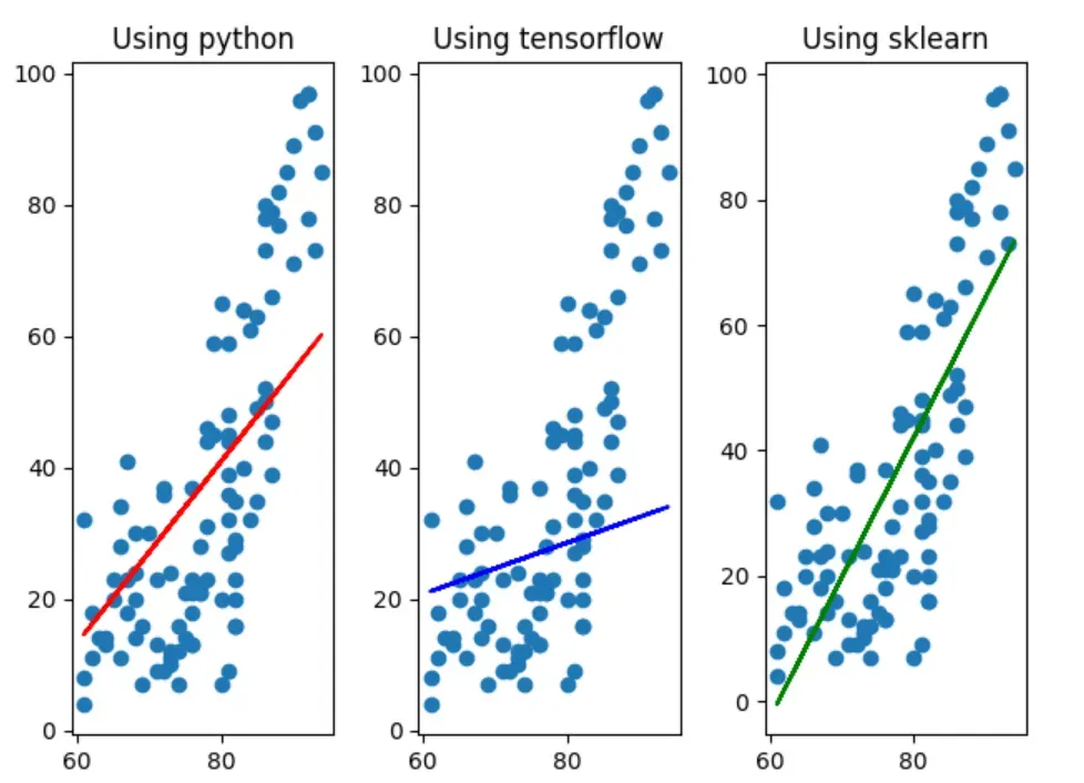
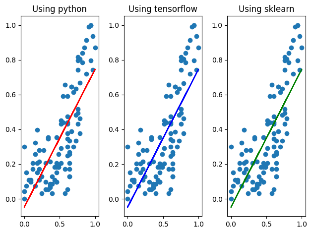
전처리를 진행하지 않은 그래프(위)와 방금 전처리를 진행한 후 구한 값으로 그린 그래프(아래)를 비교해보면, sklearn으로 구현한 모델과 거의 비슷해 진 것으로 보아 데이터 전처리의 중요성을 직관적으로 확인해 볼 수 있다.