Lecture 14. Expectation-Maximization Algorithms

cryptnomy·2022년 11월 25일

ML cs229 machine learning

CS229: Machine Learning

목록 보기

14/18

Lecture video link: https://youtu.be/rVfZHWTwXSA

Outline

Unsupervised learning
K-means clustering
Mixture of Gaussian
EM (Expectation-Maximization) algorithm
Derivation of GM

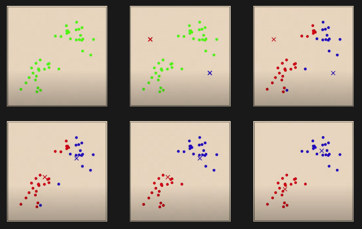
What happens during K-means clustering:

(Source: https://youtu.be/rVfZHWTwXSA?t=2m40s)

K-means Clustering

Data: $\{x^{(1)},\cdots,x^{(m)}\}$

Initialize cluster centroids $\mu_1,\cdots,\mu_k\in\mathbb{R}^d$ randomly.
Repeat until convergence:
1. Set $c^{(i)}:=\argmin\limits_j||x^{(i)}-\mu_j||$
  
  (”color the points”).
2. For $j=1,\cdots,k,$
  $\mu_j:=\frac{\sum\limits_{i=1}^m1\{c^{(i)}=j\}x^{(i)}}{\sum\limits_{i=1}^m1\{c^{(i)}=j\}}$
  (”moves the cluster centroids”).

J(\underset{\mathclap{\substack{\uparrow\\\text{assignments}}}}{c},\overset{\mathclap{\substack{\text{centroids}\\\downarrow}}}{\mu})=\sum_{i=1}^m||x^{(i)}-\mu_{c^{(i)}}||^2

Density estimation

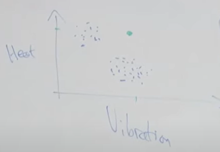
For aircraft engine,

(Source: https://youtu.be/rVfZHWTwXSA?t=17m42s)

Anomaly detection

→ Model $p(x)$

$p(x)<\epsilon\Rightarrow\text{anomaly}$ .

Mixture of Gaussians model

Problem: When applying an algorithm very similar to GDA to fit a model, the problem with this density estimation problems is that you don’t know which example actually came from which Gaussian.

→ EM algorithm comes in.

Suppose there’s a latent (hidden/unobserved) random variable $z$ , and $x^{(i)},z^{(i)}$ are distributed

p(x^{(i)},z^{(i)})=p(x^{(i)}|z^{(i)})p(z^{(i)})

where $z^{(i)}\sim\text{Multinomial}(\phi)$ and

x^{(i)}|z^{(i)}=j\sim\mathcal{N}(\mu_j,\Sigma_j).

If we knew the $z^{(i)}$ ’s, we can use MLE:

\begin{aligned}l(\phi,\mu,\Sigma)&=\sum_{i=1}^m\log p(x^{(i)},z^{(i)};\phi,\mu,\Sigma)\\ \phi_j&=\frac{1}{m}\sum_{i=1}^m1\{z^{(i)}=j\}\\ \mu_j&=\frac{\sum\limits_{i=1}^m1\{z^{(i)}=j\}x^{(i)}}{\sum\limits_{i=1}^m1\{z^{(i)}=j\}}\\ \Sigma_j&=\frac{\sum\limits_{i=1}^m1\{z^{(i)}=j\}(x^{(i)}-\mu_j)(x^{(i)}-\mu_j)^T}{\sum\limits_{i=1}^m1\{z^{(i)}=j\}}.\end{aligned}

EM (expectation-maximization)

E-step (Guess value of $z^{(i)}$ ’s):

Set

\begin{aligned}w^{(i)}_j&=p\left(z^{(i)}=j|x^{(i)};\phi,\mu,\Sigma\right)\\&=\frac{p(x^{(i)}|z^{(i)}=j)p(z^{(i)}=j)}{\sum\limits_{l=1}^kp(x^{(i)}|z^{(i)}=l)p(z^{(i)}=l)}\end{aligned}

where

p(x^{(i)}|z^{(i)}=j)=\frac{1}{(2\pi)^{n/2}|\Sigma_j|^{1/2}}\exp\left(-\frac{1}{2}(x^{(i)}-\mu_j)\Sigma_j^{-1}(x^{(i)}-\mu_j)^T\right)\\p(z^{(i)}=j)=\phi_j\;\;\;\;\;z\sim\text{Multinomial}(\phi_j)

for every $i,j$ .

M-step:

\begin{aligned}\phi_j&\leftarrow\frac{1}{m}\sum_{i=1}^mw_j^{(i)}\\ \mu_j&\leftarrow\frac{\sum\limits_{i=1}^mw_j^{(i)}x^{(i)}}{\sum\limits_{i=1}^mw_j^{(i)}}\\ \Sigma_j&\leftarrow\frac{\sum\limits_{i=1}^mw_j^{(i)}(x^{(i)}-\mu_j)(x^{(i)}-\mu_j)^T}{\sum\limits_{i=1}^mw_j^{(i)}}. \end{aligned}

$w_j^{(i)}$ is how much $x^{(i)}$ is assigned to the $\mu_j$ Gaussian.

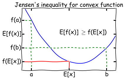
Jensen’s inequality

Let $f$ be a convex function on $\mathbb R$ (e.g., $f’’(x)>0$ ).

Let $X$ e a random variable. Then

f(\mathbb EX)\le\mathbb E[f(X)].

(Source: https://people.duke.edu/~ccc14/cspy/14_ExpectationMaximization.html)

Further, if $f’’(x)>0$ ( $f$ is strictly convex), then

\mathbb E[f(X)]=f(\mathbb EX)\Longleftrightarrow X\;\text{is a constant}.

Have model for $p(x,z;\theta)$ .

Only observe $x$ .

\begin{aligned}l(\theta)&=\sum_{i=1}^m\log p(x^{(i)};\theta)\\&=\sum_{i=1}^m\sum_{z^{(i)}}\log p(x^{(i)},z^{(i)};\theta)\end{aligned}

Want: $\argmax\limits_\theta l(\theta)$ .

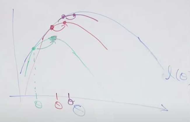
(Source: https://youtu.be/rVfZHWTwXSA?t=1h3m17s)

E-step: Construct a lower bound for $\theta$ at $j^{th}$ iteration. Draw the green curve in the figure.

M-step: Find the maximum of the green curve and update $\theta$ to the maximum.

EM algorithm only does converge to local optimum.

\begin{aligned} &\max_\theta\sum_i\log p(x^{(i)};\theta)\\ &=\sum_i\log\sum_{z^{(i)}}p(x^{(i)},z^{(i)};\theta)\\ &=\sum_i\log\sum_{z^{(i)}}Q_i(z^{(i)})\left[\frac{p(x^{(i)},z^{(i)};\theta)}{Q_i(z^{(i)})}\right]\\ &=\sum_i\log\mathbb E_{z^{(i)}\sim Q_i}\left[\frac{p(x^{(i)},z^{(i)};\theta)}{Q_i(z^{(i)})}\right]\\ &\ge\sum_i\mathbb E_{z^{(i)}\sim Q_i}\left[\log\frac{p(x^{(i)},z^{(i)};\theta)}{Q_i(z^{(i)})}\right]\\ &=\sum_i\sum_{z^{(i)}}Q_i(z^{(i)})\log\frac{p(x^{(i)},z^{(i)};\theta)}{Q_i(z^{(i)})} \end{aligned}

where $Q_i(z^{(i)})$ is a probability distribution, i.e., $\sum\limits_{z^{(i)}}Q_i(z^{(i)})=1$ .

On a given iteration of EM (with parameter $\theta$ ), we want:

\log\mathbb E_{z^{(i)}\sim Q_i}\left[\frac{p(x^{(i)},z^{(i)};\theta)}{Q_i(z^{(i)})}\right]=\mathbb E_{z^{(i)}\sim Q_i}\left[\log\frac{p(x^{(i)},z^{(i)};\theta)}{Q_i(z^{(i)})}\right].

For the above equation to hold, we need

\frac{p(x^{(i)},z^{(i)})}{Q_i(z^{(i)})}=\text{constant}.

Set $Q_i(z^{(i)})\propto p(x^{(i)},z^{(i)};\theta)$

\begin{aligned} \sum_{z^{(i)}}&Q_i(z^{(i)})=1\\ Q_i(z^{(i)})&=\frac{p(x^{(i)},z^{(i)};\theta)}{\sum\limits_{z^{(i)}}p(x^{(i)},z^{(i)};\theta)}\\ &=p(z^{(i)}|x^{(i)};\theta). \end{aligned}

Summary

E-step:

Set

Q_i(z^{(i)}):=p(z^{(i)}|x^{(i)};\theta).

M-step:

\theta:=\argmax_\theta\sum_i\sum_{z^{(i)}}Q_i(z^{(i)})\log\frac{p(x^{(i)},z^{(i)};\theta)}{Q_i(z^{(i)})}.

cryptnomy

이전 포스트

Lecture 13. Debugging ML Models and Error Analysis

다음 포스트