딥러닝 - Tensorflow: 프레임워크

1. 딥러닝의 기본 프레임워크

• Data Acquisition: 데이터 취득
• Preprocessing: 데이터 검증, 전처리 및 증강
• Modeling: 모델 설계
• Evaluation: 학습과정 추적, 후처리 및 모델 검증

---

2. Tensorflow 기반 구현

2-1. Data Acquisition

• 필요한 데이터 로드 후 shape, dtype 확인 필수

import tensorflow as tf
import numpy as np
import matplotlib.pyplot as plt
import pandas as pd

# Tensorflow 제공 MNIST 데이터셋
# 숫자 손글씨 이미지에 대한 데이터와 라벨 정보 포함
(train_x, train_y), (test_x, test_y) = tf.keras.datasets.mnist.load_data()

# shape 확인
print(train_x.shape, train_y.shape, test_x.shape, test_y.shape)
# (60000, 28, 28) (60000,) (10000, 28, 28) (10000,)

# dtype 확인
print(train_x.dtype, train_y.dtype, test_x.dtype, test_y.dtype)
# uint8 uint8 uint8 uint8

• 훈련 데이터 들여다보기

# 첫번째 데이터를 샘플로 추출
samp = train_x[0]
print(samp.shape) # (28, 28)

# 이미지 출력
plt.figure(figsize=(3, 3))
plt.imshow(samp, cmap='gray')
plt.show()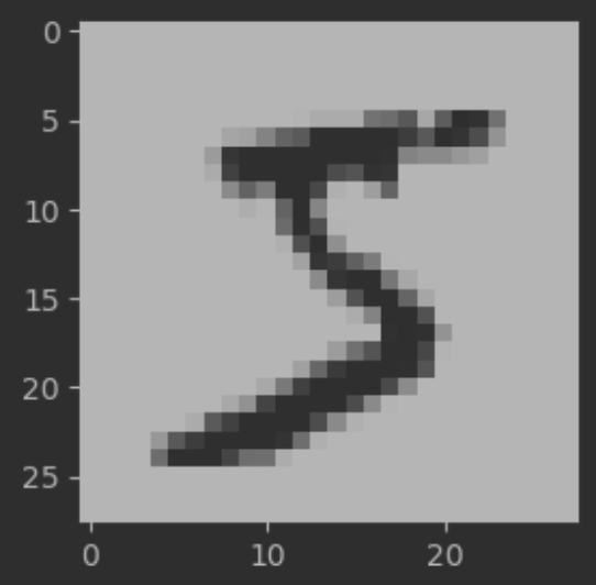

• 정답 데이터 들여다보기

# 0~9 까지의 숫자가 대체로 고르게 포함되어 있음
print(pd.Series(train_y).value_counts().sort_index())
# 0    5923
# 1    6742
# 2    5958
# 3    6131
# 4    5842
# 5    5421
# 6    5918
# 7    6265
# 8    5851
# 9    5949

2-2. Preprocessing

• 데이터 정합성 검증

# 이미지 데이터 특성상 필셀 값이 유효한지 확인
def pixel_validator(x):
    return 255 >= x.max() and 0 <= x.min()
    
train_x_res = [pixel_validator(x) for x in train_x]
text_x_res = [pixel_validator(x) for x in test_x]
print(sum(train_x_res), sum(text_x_res)) # 60000 10000

• 데이터 스케일링

# 0~1 사이의 값을 갖도록 변환
def scaler(x):
	return (x/255.0).astype("float32")
    
train_x_sc = scaler(train_x)
test_x_sc = scaler(test_x)

• 데이터 Flattening

# 딥러닝에 적합하도록 이미지의 shape 변환
print(train_x_sc.shape) # (60000, 28, 28)
print(test_x_sc.shape) # (10000, 28, 28)

train_x_sc_flat = train_x_sc.reshape(60000, -1)
test_x_sc_flat = test_x_sc.reshape(10000, -1)
print(train_x_sc_flat.shape) # (60000, 784)
print(test_x_sc_flat.shape) # (10000, 784)

• 데이터 Encoding

# 정답 데이터가 0~9의 Multi-class로 이루어져 있음
# 딥러닝에 적합하도록 One-Hot Encoding 실시
train_y_ohe = tf.keras.utils.to_categorical(train_y, 10).astype("float32")
test_y_ohe = tf.keras.utils.to_categorical(test_y, 10).astype("float32")
print(train_y_ohe[0])
# [0. 0. 0. 0. 0. 1. 0. 0. 0. 0.]
# 샘플 데이터에서 확인하였듯이, 인코딩 결과가 숫자 5를 나타내고 있음

2-3. Modeling

• 모델 정의

from tensorflow.keras import Sequential
from tensorflow.keras.layers import Dense, Activation

INPUT_DIM = train_x_sc_flat.shape[1]
model = Sequential()
model.add(Dense(32, input_dim=INPUT_DIM)) # 784개 데이터를 32개로 압축
model.add(Activation("sigmoid")) # 각 노드의 출력값을 0과 1 사이로 변환
model.add(Dense(10)) # 32개 데이터를 10개(정답 데이터와 동일)로 압축
model.add(Activation("softmax")) # 각 노드의 출력값의 총합이 1이 되도록 변환
model.summary()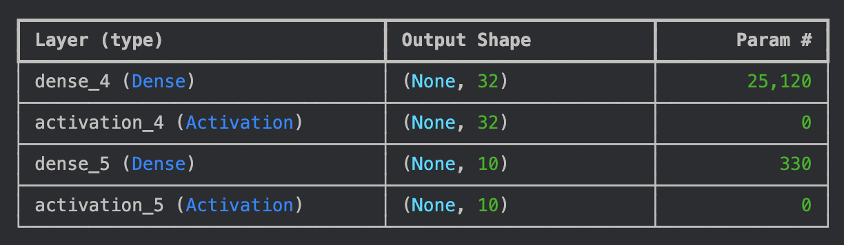

• 모델 컴파일

from tensorflow.keras.optimizers import SGD
from tensorflow.keras.losses import categorical_crossentropy

opt = SGD(learning_rate=0.03) # 최적화함수 (가중치와 편향 업데이트)
loss = categorical_crossentropy # 손실함수 (오차 측정)

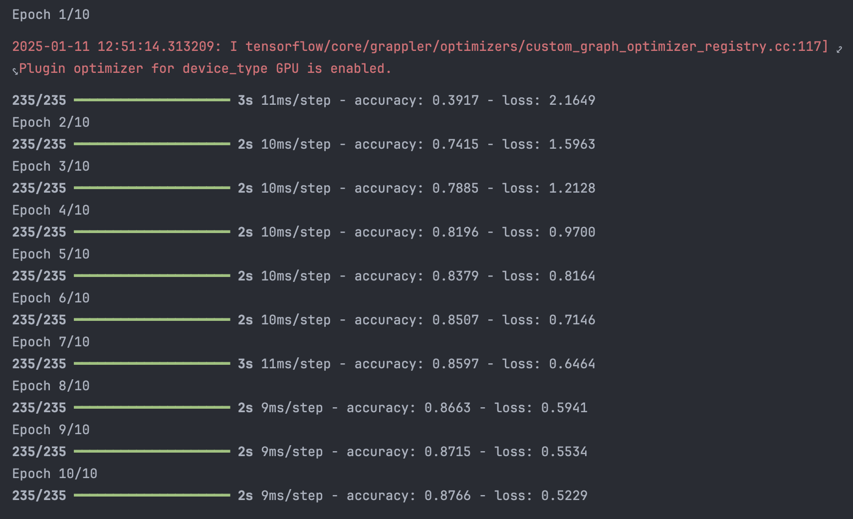
model.compile(optimizer=opt, loss=loss, metrics=["accuracy"])

• 모델 학습

# 60,000개 데이터 / 256개 배치 사이즈 = 1 epoch 당 235번 업데이트 실시
hist = model.fit(train_x_sc_flat, train_y_ohe, epochs=10, batch_size=256)

2-4. Evaluation

• 학습과정 확인

fig, ax1 = plt.subplots(figsize=(5, 3))
ax2 = ax1.twinx() # 이중축 설정
ax1.plot(np.arange(1, 11, 1), hist.history['loss'], label="Loss", c="grey")
ax1.set_xlabel("Epoch")
ax1.set_ylabel("Loss")
ax2.plot(np.arange(1, 11, 1), hist.history['accuracy'], label="Acc.", c="red")
ax2.set_ylim([0, 1])
ax2.set_ylabel("Acc.")
fig.suptitle("Loss and Accuracy")
fig.legend(bbox_to_anchor=(0.88, 0.7))
plt.show()
# Epochs 수를 더 늘려, 손실이 수렴되는지 봐도 될 것으로 예상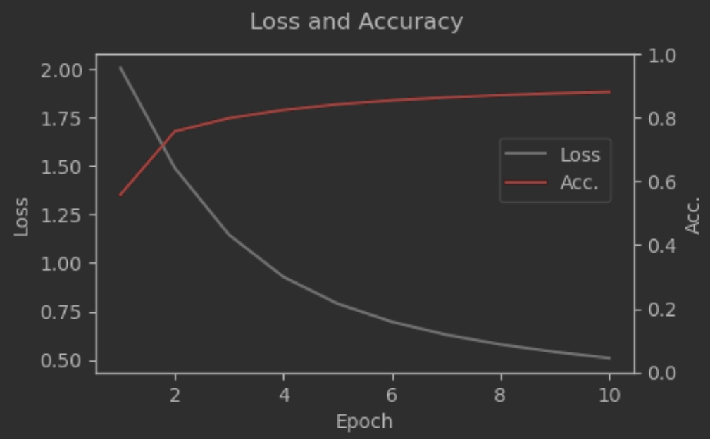

• 모델 검증

model.evaluate(test_x_sc_flat, test_y_ohe)
# [0.48081356287002563, 0.8902999758720398]
# Loss는 약 0.48, Accuracy는 약 0.89 정도 해당

• 후처리

# 예측 수행 시 softmax 함수에 따라 각 클래스에 속할 확률이 반환됨
test_y_pred = model.predict(test_x_sc_flat)
print(test_y_pred[0])
# [4.0102964e-03 9.0400281e-04 1.2402087e-03 5.5419970e-03 6.8208005e-04
#  3.1641328e-03 9.4013871e-05 9.5357978e-01 1.1781736e-03 2.9605296e-02]

# np.argmax() 함수를 통해 각 클래스로 변환 작업 적용
test_y_pred = test_y_pred.argmax(axis=1)
test_y_pred[0] # 7

# 이미지 확인 결과 정확히 예측하였음을 확인
samp = test_x[0]
plt.figure(figsize=(3, 3))
plt.imshow(samp, cmap='gray')
plt.show()

---

*이 글은 제로베이스 데이터 취업 스쿨의 강의 자료 일부를 발췌하여 작성되었습니다.