Bitcoin hash-rate 예측 1차 Defense

https://www.kaggle.com/geunyeongju/defense-baseline-code

데이터 로드

train = pd.read_csv('/kaggle/input/sejongai-hashrate/train.csv')
test = pd.read_csv('/kaggle/input/sejongai-hashrate/test.csv')
sample = pd.read_csv('/kaggle/input/sejongai-hashrate/submit_sample.csv')

모듈 임포트 및 GPU 사용

import numpy as np
import pandas as pd
import torch
import torch.nn as nn
import torch.optim as optim
import random
from sklearn.preprocessing import MinMaxScaler

device ='cuda' if torch.cuda.is_available() else 'cpu'

random.seed(777)
torch.manual_seed(777)
if device == 'cuda' :
  torch.cuda.manual_seed_all(777)

device

데이터 파싱

x_train = train.iloc[:,1:-1]
x_train['Timestamp'] = x_train['Timestamp'].str.split('/').str[0].astype(int)
x_test = test.iloc[:,1:]
x_test['Timestamp'] = x_test['Timestamp'].str.split('/').str[0].astype(int)
y_train = train.iloc[:,-1]


sc = StandardScaler()
x_train = sc.fit_transform(x_train)
x_test = sc.transform(x_test)

x_train = torch.FloatTensor(x_train).to(device)
x_test = torch.FloatTensor(x_test).to(device)
y_train = torch.FloatTensor(y_train).reshape(-1,1).to(device)

년도와 월,일을 '/' 단위로 구분하여 월 다시 뽑아 Timestamp열에 넣어주어 학습 데이터를 재 가공하였습니다.

데이터 확인

# train data
print(x_train[:5])
print(x_train.shape)
print(y_train[:5])
print(y_train.shape)

# test data
print(x_test[:3])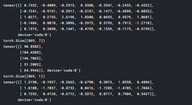

모델 정의

class NN(torch.nn.Module):
    def __init__(self):
        super(NN,self).__init__()
        
        self.linear1 = nn.Linear(7,512,bias=True)
        self.linear2 = nn.Linear(512,256,bias=True)
        self.linear3 = nn.Linear(256,512,bias=True)
        self.linear4 = nn.Linear(512,64,bias=True)
        self.linear5 = nn.Linear(64,32,bias=True)
        self.linear6 = nn.Linear(32,1,bias=True)
        self.relu = nn.ReLU()
        
        torch.nn.init.orthogonal_(self.linear1.weight)
        torch.nn.init.orthogonal_(self.linear2.weight)
        torch.nn.init.orthogonal_(self.linear3.weight)
        torch.nn.init.orthogonal_(self.linear4.weight)
        torch.nn.init.orthogonal_(self.linear5.weight)
        torch.nn.init.orthogonal_(self.linear6.weight)
        
    def forward(self,x):
        out = self.linear1(x)
        out = self.relu(out)
        out = self.linear2(out)
        out = self.relu(out)
        out = self.linear3(out)
        out = self.relu(out)
        out = self.linear4(out)
        out = self.relu(out)
        out = self.linear5(out)
        out = self.relu(out)
        out = self.linear6(out)
        return out

열이 하나 더 추가되어 인풋은 7로 설정하였습니다.

학습 파라미터 설정

model = NN().to(device)
optimizer = optim.Adam(model.parameters(), lr=15e-5)
loss = nn.MSELoss().to(device)
epochs = 1500
model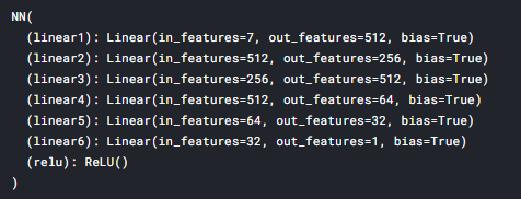

과적합을 막기 위해서 epochs를 1500까지 줄였을 때 제일 높은 성능이 나오는 것을 확인했습니다.
또한 learning rate도 변경해주었습니다.

모델 학습

model.train()
plt_los = []
train_total_batch = len(x_train)
for epoch in range(epochs+1) : 
    avg_cost = 0
    model.train()

    hypothesis = model(x_train) 
    cost = loss(hypothesis,y_train) 
    
    optimizer.zero_grad() 
    cost.backward()
    optimizer.step() 
    avg_cost += cost / train_total_batch
    plt_los.append([avg_cost.item()])
    if epoch%100==0:
        print('Epoch : {}, Cost : {}'.format(epoch, avg_cost.item()))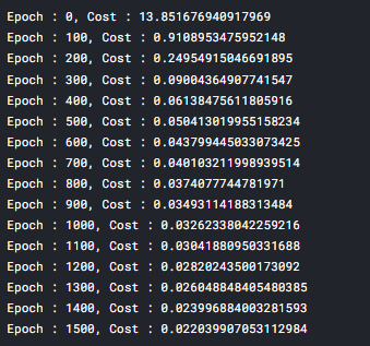

Plot

import matplotlib.pyplot as plt

def plot(loss_list: list, ylim=None, title=None) -> None:
    bn = [i[0] for i in loss_list]

    plt.figure(figsize=(10, 10))
    plt.plot(bn, label='avg_cost')
    if ylim:
        plt.ylim(ylim)

    if title:
        plt.title(title)
    plt.legend()
    plt.grid('on')
    plt.show()
    
plot(plt_los , [0.0, 1.0], title='Loss at Epoch')
print(avg_cost.item())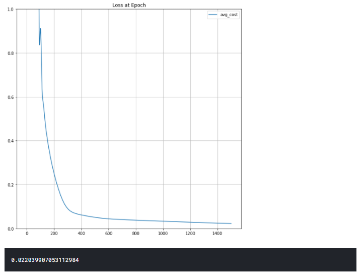

plot 함수를 정의하여 cost 값을 시각화 하여 잘 학습되었다는 것을 확인했습니다.

예측 값 도출 및 제출

model.eval()
with torch.no_grad():
    y_pred = model(x_test)
sample['hash-rate'] = y_pred.cpu().numpy()
sample.to_csv('submit_sample.csv',index=False)
sample