Kernel Support Vector Classifier (KSVC)

Introduction

Kernel Support Vector Classifier (SVC) extends the Support Vector Machine (SVM) concept to handle non-linear data by applying kernel functions. This approach allows the algorithm to operate in a transformed feature space without explicitly computing the transformation, enabling efficient classification of complex and non-linearly separable data sets. Kernel SVC is widely recognized for its robustness and versatility in various machine learning tasks.

Background and Theory

The core idea behind Kernel SVC is to map the input data into a higher-dimensional space where it becomes linearly separable, using a kernel function. This process facilitates finding a hyperplane in the transformed space that can separate the data points based on their class labels with a maximal margin while minimizing classification error.

How the Algorithm Works

Steps

1. Mapping to Higher-Dimensional Space: Implicitly transform the input data into a higher-dimensional space using a kernel function.
2. Optimal Hyperplane Identification: In the transformed feature space, identify the optimal hyperplane that separates the classes with the largest margin.
3. Support Vector Identification: Determine the support vectors that are critical to defining the hyperplane.
4. Decision Function Derivation: Derive a decision function based on the support vectors and the kernel function to classify new instances.

Mathematical Formulation

Given a dataset of $n$ points $(\mathbf{x}_i, y_i)$, where $\mathbf{x}_i$ is an input feature vector and $y_i \in \{-1, 1\}$ is the class label, the goal is to find a function $f(\mathbf{x})$ that can predict the class label of a new instance.

The decision function in the context of kernel SVC is formulated as:

where:

• $K(\mathbf{x}_i, \mathbf{x})$ is the kernel function, computing the dot product between $\mathbf{x}_i$ and $\mathbf{x}$ in the transformed feature space.
• $\alpha_i$ are Lagrange multipliers obtained by solving the dual optimization problem.
• $b$ is the bias term.

The optimization problem maximizes the margin between classes while minimizing classification error, subject to certain constraints related to the data labels and the Lagrange multipliers.

Commonly used kernel functions include:

• Linear: $K(\mathbf{x}_i, \mathbf{x}_j) = \mathbf{x}_i^T \mathbf{x}_j$
• Polynomial: $K(\mathbf{x}_i, \mathbf{x}_j) = (\gamma \mathbf{x}_i^T \mathbf{x}_j + r)^d$
  where $\gamma$, $r$, and $d$ are kernel parameters.
  
• Radial Basis Function (RBF): $K(\mathbf{x}_i, \mathbf{x}_j) = \exp(-\gamma \|\mathbf{x}_i - \mathbf{x}_j\|^2)$
  where $\gamma$ is a kernel parameter.
  

Implementation

Parameters

• C: float, default = 1.0
  Regularization parameter
  
• deg: int, default = 3
  Polynomial Degree for ‘poly’ kernel
  
• gamma: float, default = 1.0
  Shape parameter of Gaussian curve for ‘rbf’ kernel
  
• coef: float, default = 1.0
  Coefficient for ‘poly’, ‘sigmoid’ kernel
  
• learning_rate: float, default = 0.001
  Step-size for gradient descent update
  
• max_iter: int, default = 1000
  Number of iteration
  
• batch_size: int, default = 100
  Size of the batch for batch-based learning
  
• kernel: KernelUtil.func_type, default = ‘rbf’
  Type of kernel
  

Examples

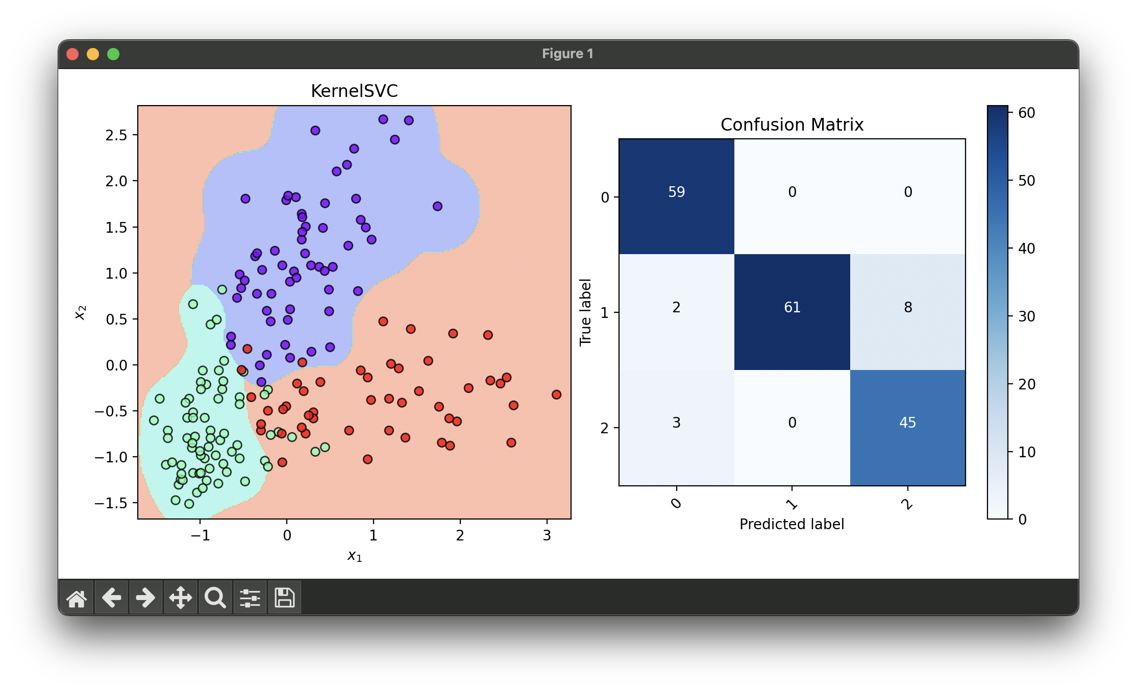
Test on wine dataset with dimensionality reduction via RFE and tuning with RandomizedSearchCV:

from luma.classifier.svm import KernelSVC
from luma.classifier.naive_bayes import GaussianNaiveBayes
from luma.preprocessing.scaler import StandardScaler
from luma.reduction.selection import RFE
from luma.model_selection.split import TrainTestSplit
from luma.model_selection.search import RandomizedSearchCV
from luma.visual.evaluation import DecisionRegion, ConfusionMatrix

from sklearn.datasets import load_wine
import matplotlib.pyplot as plt
import numpy as np


X, y = load_wine(return_X_y=True)

X_train, X_test, y_train, y_test = TrainTestSplit(X, y,
                                                  test_size=0.3,
                                                  random_state=42).get

sc = StandardScaler()
X_train_std = sc.fit_transform(X_train)
X_test_std = sc.fit_transform(X_test)

rfe = RFE(estimator=GaussianNaiveBayes(),
          n_features=2,
          step_size=1,
          cv=5,
          random_state=42,
          verbose=True)

rfe.fit(X_train_std, y_train)
X_train_rfe = rfe.transform(X_train_std)
X_test_rfe = rfe.transform(X_test_std)

param_dist = {'C': np.logspace(-3, 2, 5),
              'deg': range(2, 10),
              'gamma': np.logspace(-3, 1, 5),
              'learning_rate': np.logspace(-3, -1, 5),
              'kernel': ['poly', 'rbf', 'sigmoid']}

rand = RandomizedSearchCV(estimator=KernelSVC(),
                          param_dist=param_dist,
                          max_iter=20,
                          cv=5,
                          refit=True,
                          random_state=42,
                          verbose=True)

rand.fit(X_train_rfe, y_train)
ksvc_best = rand.best_model

X_concat = np.concatenate((X_train_rfe, X_test_rfe))
y_concat = np.concatenate((y_train, y_test))

fig = plt.figure(figsize=(10, 5))
ax1 = fig.add_subplot(1, 2, 1)
ax2 = fig.add_subplot(1, 2, 2)

dec = DecisionRegion(ksvc_best, X_concat, y_concat)
dec.plot(ax=ax1)

conf = ConfusionMatrix(y_concat, ksvc_best.predict(X_concat))
conf.plot(ax=ax2, show=True)

# Best params: {
#     'C': 0.31622776601683794, 
#     'deg': 9, 
#     'gamma': 10.0, 
#     'learning_rate': 0.001, 
#     'kernel': 'rbf'
# }
# Best score: 0.912

Applications and Use Cases

• Image Recognition: Classifying images by recognizing patterns and features that are not linearly separable.
• Text Classification: Categorizing documents or messages into different topics based on content similarity.
• Bioinformatics: Classifying proteins or genes into functional families based on their sequence or structure features.
• Customer Segmentation: Grouping customers based on purchasing behavior and preferences for targeted marketing strategies.

Strengths and Limitations

• Strengths
  • Ability to handle non-linear data effectively through the use of kernel functions.
  • Flexibility in choosing the kernel function to best suit the problem at hand.
  • Robustness to overfitting, particularly in high-dimensional spaces, due to the maximization of the margin.
• Limitations
  • Selection of the kernel function and its parameters can be challenging and requires careful tuning.
  • Computational complexity increases with the size of the dataset, making it less efficient for very large datasets.
  • The algorithm's performance is sensitive to feature scaling.

Advanced Topics and Further Reading

• Kernel Selection and Parameter Tuning: Strategies for selecting the appropriate kernel function and tuning its parameters using cross-validation and grid search techniques.
• Multi-Class Classification: Adapting kernel SVC for multi-class classification problems using strategies like one-vs-one or one-vs-rest approaches.
• Feature Engineering and Dimensionality Reduction: Techniques to enhance model performance and reduce computational complexity, such as Principal Component Analysis (PCA) or feature selection methods.

References

1. Schölkopf, B., & Smola, A. J. (2001). Learning with Kernels: Support Vector Machines, Regularization, Optimization, and Beyond. MIT Press.
2. Vapnik, V. N. (1998). Statistical Learning Theory. Wiley.
3. Cristianini, N., & Shawe-Taylor, J. (2000). An Introduction to Support Vector Machines and Other Kernel-based Learning Methods. Cambridge University Press.
4. Burges, C. J. C. (1998). A tutorial on support vector machines for pattern recognition. Data Mining and Knowledge Discovery, 2(2), 121-167.