Adaptive Spectral Clustering

Introduction

Adaptive Spectral Clustering enhances the spectral clustering framework by dynamically adjusting the algorithm's parameters, notably the similarity metric, to better fit the data's inherent structure. This adaptiveness allows for more accurate discovery of clusters, particularly in complex or heterogeneous datasets.

Background and Theory

Traditional spectral clustering techniques require predefined parameters, such as the number of clusters or the scale of the similarity measure, which can be suboptimal without prior knowledge of the dataset's structure. Adaptive Spectral Clustering addresses this by iteratively refining these parameters based on the data, leading to a more flexible and effective clustering process.

Mathematical Foundations

Adaptive Spectral Clustering involves constructing a similarity graph $G = (V, E)$, where $V$ represents data points and $E$ represents edges weighted by a similarity function $W_{ij}$ between data points $x_i$ and $x_j$. Unlike static methods, adaptive approaches modify $W_{ij}$ during the clustering process to better capture the data's natural divisions.

The adaptive similarity measure can be defined as:

where $\sigma_{ij}$ is an adaptive scale parameter that adjusts based on local or global data characteristics, enhancing the algorithm's ability to identify clusters of varying densities and shapes.

The degree matrix $D$ and the normalized Laplacian $L_{\text{norm}}$ are calculated as usual, but with the adaptive $W_{ij}$ values:

Procedural Steps

1. Initial Similarity Graph Construction: Create an initial similarity graph $G$ using a preliminary estimation of the similarity measure.
2. Adaptive Parameter Adjustment: Refine the similarity measures $W_{ij}$ by considering the local density or other data-driven metrics, updating $\sigma_{ij}$ accordingly.
3. Laplacian and Eigenvalue Decomposition: Compute the adaptive normalized Laplacian $L_{\text{norm}}$ and perform eigenvalue decomposition to obtain its eigenvalues and eigenvectors.
4. Low-Dimensional Mapping: Map each data point to a lower-dimensional space using the eigenvectors corresponding to the smallest non-zero eigenvalues, as in standard spectral clustering.
5. Clustering in Reduced Space: Apply a clustering algorithm to the points in the new feature space to identify clusters.

Mathematical Formulations

The adaptiveness comes from the iterative refinement of $\sigma_{ij}$, which can be updated based on local density estimates or other criteria, such as:

where $\sigma_i$ and $\sigma_j$ are local scale parameters for points $x_i$ and $x_j$, calculated based on the distances to their $k$-th nearest neighbors or through other local density estimation techniques.

The eigenvalue problem for the adaptive normalized Laplacian remains:

with the goal of finding a partition that minimizes the normalized cut, adapting the graph structure iteratively to reveal the underlying cluster structure more effectively.

Implementation

Parameters

• gamma: float, default = 1.0
  Scaling factor for Gaussian kernel
  
• max_cluster: int, default = 10
  Upper-bound of the number of clusters to estimate
  

Examples

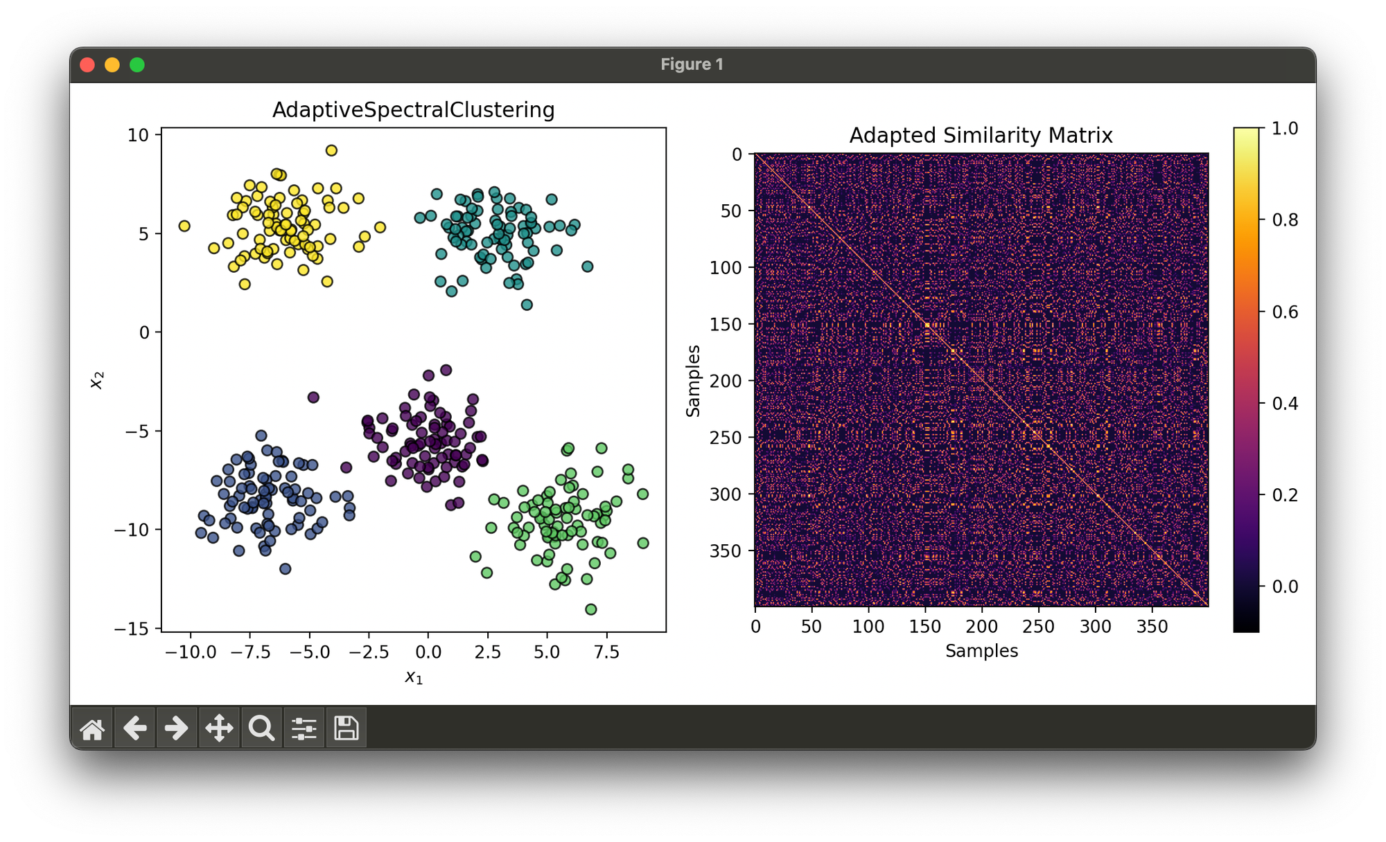
Test on synthesizd dataset with 5 blobs:

from luma.clustering.spectral import AdaptiveSpectralClustering
from luma.metric.clustering import SilhouetteCoefficient
from luma.visual.evaluation import ClusterPlot

from sklearn.datasets import make_blobs
import matplotlib.pyplot as plt

X, y = make_blobs(n_samples=400, 
                  centers=5,  
                  cluster_std=1.5, 
                  random_state=10)

asp = AdaptiveSpectralClustering(gamma=0.1, max_clusters=10)
asp.fit(X)

fig = plt.figure(figsize=(10, 5))
ax1 = fig.add_subplot(1, 2, 1)
ax2 = fig.add_subplot(1, 2, 2)

clst = ClusterPlot(asp, X, cmap='viridis')
clst.plot(ax=ax1)

sil = SilhouetteCoefficient(X, asp.labels)
sil.plot(ax=ax2, show=True)

Applications

• Complex Data Clustering: Particularly useful for datasets with clusters of varying densities and non-linear boundaries.
• Image and Vision: Adaptive techniques can better segment images with heterogeneous textures or lighting conditions.
• Biological Data Analysis: Identifies functional groups or patterns within genetic or protein interaction networks.

Strengths and Limitations

Strengths

• Flexibly adapts to the inherent structure of the data, improving cluster quality.
• Capable of handling datasets with complex geometries and varying densities.

Limitations

• Increased computational complexity due to the iterative adjustment of parameters.
• The selection of criteria for adaptively adjusting parameters can significantly influence results.

Advanced Topics

• Automatic Parameter Selection: Techniques for automatically determining optimal parameters, such as the number of clusters or the initial scale of the similarity measure.
• Integration with Deep Learning: Leveraging deep neural networks to learn adaptive similarity measures in an end-to-end manner.

References

1. Zelnik-Manor, Lihi, and Pietro Perona. "Self-tuning spectral clustering." Advances in neural information processing systems 17 (2004): 1601-1608.
2. Von Luxburg, Ulrike. "A tutorial on spectral clustering." Statistics and Computing 17, no. 4 (2007): 395-416.