Hierarchical Spectral Clustering

Introduction

Hierarchical Spectral Clustering combines the principles of hierarchical clustering with spectral methods to analyze data structures at multiple scales. This approach allows for the exploration of data clustering in a manner that uncovers nested relationships between clusters, offering a versatile framework for understanding complex datasets.

Background and Theory

Hierarchical Spectral Clustering extends the spectral clustering methodology by iteratively applying spectral clustering in a hierarchical manner. This iterative process enables the identification of cluster structures at various levels of granularity, providing a multi-resolution analysis of the data.

Mathematical Foundations

At the core of Hierarchical Spectral Clustering is the construction and analysis of the graph Laplacian, similar to standard spectral clustering. Given a dataset $X = \{x_1, x_2, \ldots, x_n\}$, we first construct a similarity graph $G = (V, E)$, with vertices $V$ representing data points, and weighted edges $E$ representing similarities between these points. The weight of an edge $(i, j)$ is denoted by $W_{ij}$, typically calculated using a similarity measure such as the Gaussian kernel:

where $\sigma$ is a parameter that influences the scale of neighborhood relationships.

The degree matrix $D$ and the graph Laplacian $L$ are defined as in standard spectral clustering, with the normalized Laplacian $L_{\text{norm}}$ being particularly crucial for hierarchical spectral clustering:

Procedural Steps

1. Graph Construction: Create a similarity graph $G$ from the data $X$.
2. Laplacian Computation: Compute the normalized Laplacian $L_{\text{norm}}$.
3. Hierarchical Clustering:
   • Perform eigenvalue decomposition on $L_{\text{norm}}$ to find its eigenvalues and eigenvectors.
   • Use the eigenvectors corresponding to the smallest eigenvalues to map the data into a lower-dimensional space.
   • Apply a hierarchical clustering method (e.g., agglomerative clustering) on the mapped data to construct a dendrogram representing the nested cluster structure.
4. Cluster Extraction: Determine the level of granularity desired (e.g., the number of clusters) and cut the dendrogram at the corresponding depth to extract the clusters.

Mathematical Formulations

The eigenvalue decomposition of $L_{\text{norm}}$ is a critical step, leading to the eigenvalues $\lambda_1 \leq \lambda_2 \leq \ldots \leq \lambda_n$ and their corresponding eigenvectors $u_1, u_2, \ldots, u_n$. The first $k$ eigenvectors are used to form a feature matrix $U \in \mathbb{R}^{n \times k}$:

where the columns are the eigenvectors. Each row of $U$ represents a data point in the new feature space. The hierarchical clustering is then applied to these points.

The decision on the number of clusters, or the cut on the dendrogram, can be informed by analyzing the eigenvalues (the eigengap heuristic) or by leveraging domain-specific knowledge.

Implementation

Parameters

• n_clusters: int
  Number of clusters to estimate
  
• method: Literal['agglomerative', 'divisive'], default = ‘agglomerative’
  Method for hierarchical clustering
  
• linkage: Literal['single', 'complete', 'average'], default = ‘single’
  Linkage method for ‘agglomerative’ clustering
  
• gamma: float, default = 1.0
  Scaling factor for Gaussian(RBF) kernel
  

Examples

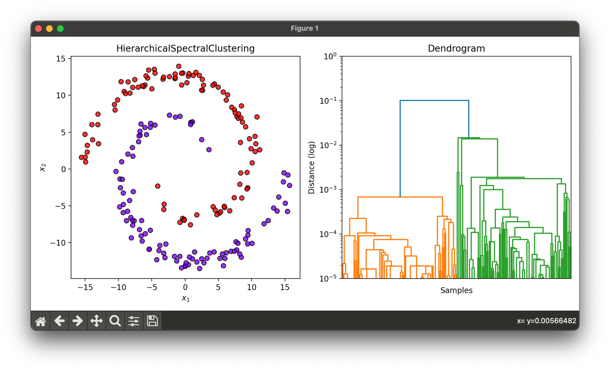
Test on synthesized dataset with 2 spirals:

from luma.clustering.spectral import HierarchicalSpectralClustering
from luma.visual.evaluation import ClusterPlot

import numpy as np
import matplotlib.pyplot as plt

def generate_spiral_dataset(points_per_spiral=100, noise=0.7):
    n = points_per_spiral
    theta = np.sqrt(np.random.rand(n)) * 2 * np.pi
    
    r_a = 2 * theta + np.pi
    data_a = np.array([np.cos(theta) * r_a, np.sin(theta) * r_a]).T
    x_a = data_a + np.random.randn(n, 2) * noise

    r_b = -2 * theta - np.pi
    data_b = np.array([np.cos(theta) * r_b, np.sin(theta) * r_b]).T
    x_b = data_b + np.random.randn(n, 2) * noise

    X = np.concatenate((x_a, x_b))
    y = np.concatenate((np.zeros(n), np.ones(n)))

    return X, y

X, y = generate_spiral_dataset()

hsp = HierarchicalSpectralClustering(n_clusters=2,
                                     method='agglomerative',
                                     linkage='single',
                                     gamma=0.5)

hsp.fit(X)

fig = plt.figure(figsize=(10, 5))
ax1 = fig.add_subplot(1, 2, 1)
ax2 = fig.add_subplot(1, 2, 2)

clst = ClusterPlot(hsp, X)
clst.plot(ax=ax1)

hsp.plot_dendrogram(ax=ax2)
ax2.set_yscale('log')
ax2.set_ylabel('Distance (log)')
ax2.set_ylim(1e-5, 1e-0)

plt.tight_layout()
plt.show()

Applications

• Network Analysis: Unveiling hierarchical community structures within social or biological networks.
• Document Clustering: Organizing collections of documents into a hierarchy of topics and subtopics.
• Image Processing: Segmenting images into hierarchical components for detailed analysis.

Strengths and Limitations

Strengths

• Provides insights into the hierarchical structure of data, which is not possible with flat clustering methods.
• Flexible in the choice of scale, allowing for detailed or broad cluster analysis.

Limitations

• Computational complexity can be high, especially for large datasets and deep hierarchical levels.
• The choice of parameters (e.g., similarity measure, $\sigma$) significantly influences the clustering results.

Advanced Topics

• Dynamic Hierarchical Clustering: Adapting the hierarchical structure as new data points are added, without recomputing the entire hierarchy.
• Multiscale Graph Partitioning: Techniques for identifying cluster structures at multiple scales simultaneously.

References

1. Von Luxburg, Ulrike. "A tutorial on spectral clustering." Statistics and Computing 17, no. 4 (2007): 395-416.
2. Shi, Jianbo, and Jitendra Malik. "Normalized cuts and image segmentation." IEEE Transactions on Pattern Analysis and Machine Intelligence 22, no. 8 (2000): 888-905.