Affinity Propagation (AP)

Introduction

Affinity Propagation (AP) is a clustering algorithm introduced by Brendan J. Frey and Delbert Dueck in 2007. Unlike traditional clustering algorithms such as k-means, which require the number of clusters to be specified in advance, Affinity Propagation determines the number of clusters based on the input data. The algorithm operates by considering all data points as potential exemplars (cluster centers) and iteratively exchanging messages between data points until a set of high-quality exemplars and corresponding clusters emerges.

Background and Theory

The fundamental idea behind Affinity Propagation is the concept of "message passing" between data points. The algorithm uses two types of messages: "responsibility" $r(i, k)$, which reflects how well-suited point $k$ is to serve as the exemplar for point $i$, and "availability" $a(i, k)$, which indicates how appropriate it would be for point $i$ to choose point $k$ as its exemplar, considering other points' preferences for $k$ as an exemplar.

Mathematical Foundations

The algorithm starts with the similarity $s(i, k)$ between pairs of data points, which is typically the negative Euclidean distance, although other metrics can be used. For point $k$ to be considered an exemplar, we also set $s(k, k)$ to a value referred to as the "preference", which can be viewed as the algorithm's input parameter that influences the number of clusters.

The "responsibility" $r(i, k)$ is updated as follows:

And the "availability" $a(i, k)$ is updated using:

For $i = k$, the availability update rule is slightly different:

These messages are iteratively exchanged until a stable set of exemplars and clusters is found.

Procedural Steps

1. Initialization: Initialize the responsibility and availability matrices to zero.
2. Update Responsibilities: For each data point, update the responsibility matrix using the formula provided above.
3. Update Availabilities: For each data point, update the availability matrix using the formula provided above.
4. Check Convergence: After several iterations, check if the decisions about exemplars remain unchanged. If they have stabilized, the algorithm has converged.
5. Identify Exemplars and Clusters: After convergence, the exemplars are identified by the points for which the sum of responsibility and availability is positive, and clusters are formed based on these exemplars.

Implementation

Parameters

• max_iter: int, default = 100
  Maximum iterations for message exchange
  
• damping: float, default = 0.7
  Balancing factor for ensuring numerical stability and convergence
  
• preference: Scalar Vector Literal['median', 'min'], default = ‘median’
  Parameter which determines the selectivity of choosing exemplars
  
• tol: float, default = None
  Early-stopping threshold
  

Properties

• Get assigned cluster labels:

  @property
  def labels(self) -> Matrix

Notes

• Self-Similarity Setting: The preference value represents the "self-similarity" of each data point. It is the value on the diagonal of the similarity matrix, which influences how likely a data point is to be chosen as an exemplar (a cluster center).
• Influencing Cluster Count: A higher preference value suggests a greater likelihood for a data point to become an exemplar, potentially leading to more clusters. Conversely, a lower preference value tends to produce fewer clusters, as fewer points are strong candidates for being exemplars.
• Default Setting: If not explicitly set, the preference is often chosen automatically based on the input data. Common practices include setting it to the median or mean of the similarity values.

Examples

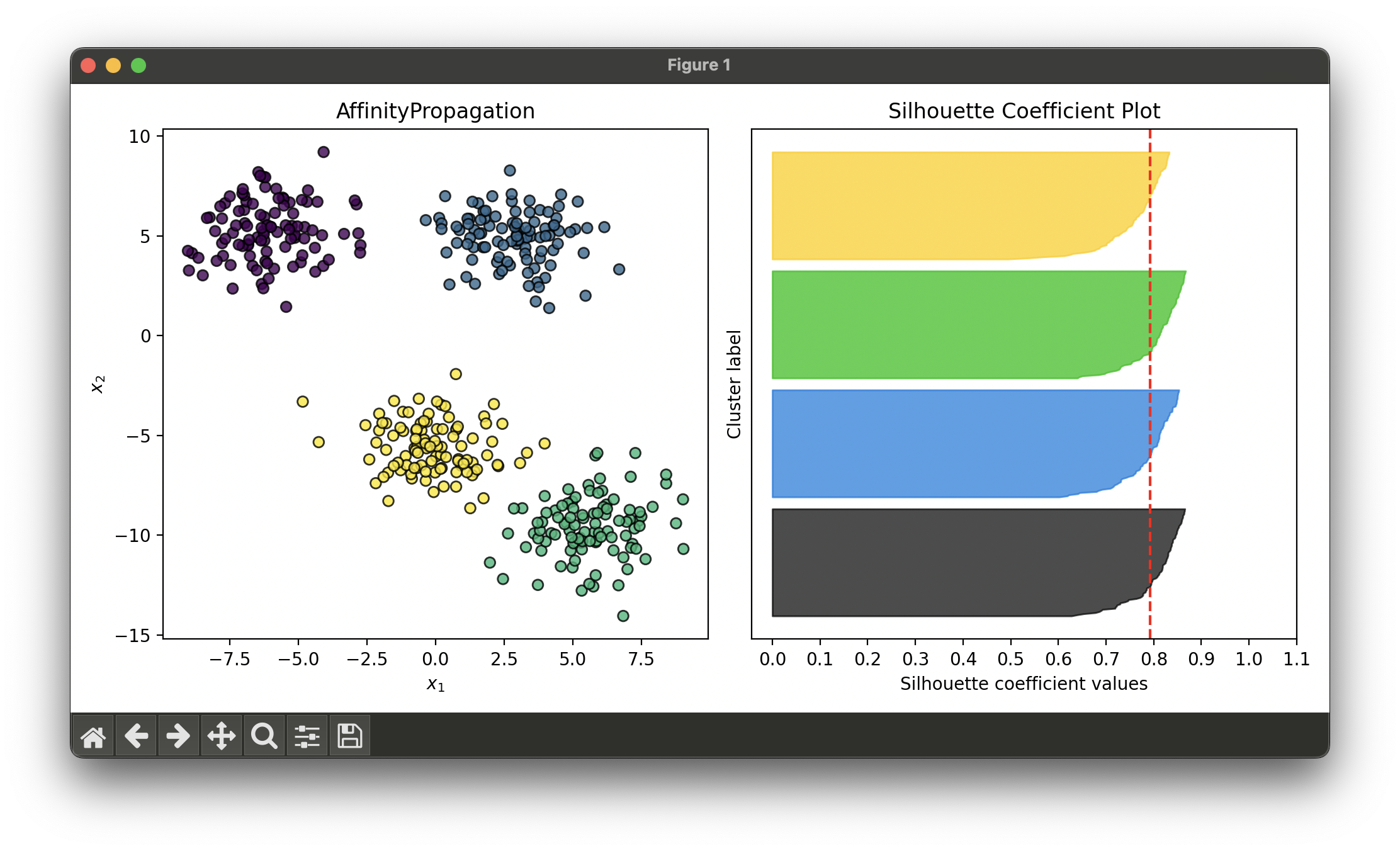
Test with synthesized dataset of 4 blobs:

from luma.clustering.affinity import AffinityPropagation
from luma.visual.evaluation import ClusterPlot
from luma.metric.clustering import SilhouetteCoefficient

from sklearn.datasets import make_blobs
import matplotlib.pyplot as plt


X, y = make_blobs(n_samples=400, 
                  cluster_std=1.5, 
                  centers=4, 
                  random_state=10)

ap = AffinityPropagation(max_iter=100,
                         damping=0.7,
                         preference='min')

ap.fit(X)

fig = plt.figure(figsize=(10, 5))
ax1 = fig.add_subplot(1, 2, 1)
ax2 = fig.add_subplot(1, 2, 2)

clst = ClusterPlot(ap, X, cmap='viridis')
clst.plot(ax=ax1)

sil = SilhouetteCoefficient(X, ap.labels)
sil.plot(ax=ax2, show=True)

Applications

• Gene Expression Analysis: Identifying groups of genes with similar expression patterns.
• Image Recognition: Clustering segments of images for object recognition.
• Market Segmentation: Grouping customers with similar preferences or behaviors.

Strengths and Limitations

Strengths

• Automatic Determination of Cluster Number: Unlike many clustering algorithms, Affinity Propagation does not require the number of clusters to be specified in advance.
• Flexibility: Works with various similarity measures, allowing it to be applied to different types of data.
• Efficiency: Often faster than other methods when identifying exemplars among thousands of data points.

Limitations

• Sensitivity to Preferences: The outcome is sensitive to the input preferences, which can sometimes make the selection of a suitable preference value challenging.
• Memory Usage: The algorithm requires the storage of a matrix of similarities, which can be prohibitive for very large datasets.

Advanced Topics

• Preference Selection Strategies: Exploring methods for selecting the preference parameter can significantly impact the algorithm's performance and the quality of the clustering.
• Scalability Improvements: Techniques for reducing memory usage and computational cost, such as sparse representation of the similarity matrix, can make Affinity Propagation more applicable to large datasets.

References

1. Frey, Brendan J., and Delbert Dueck. "Clustering by Passing Messages Between Data Points." Science 315.5814 (2007): 972-976.
2. Kriegel, Hans-Peter, et al. "A survey of clustering algorithms." Encyclopedia of Database Systems. Springer, 2009.