Gaussian Mixture Model (GMM)

Introduction

Gaussian Mixture Models (GMMs) are a probabilistic model for representing normally distributed subpopulations within an overall population. Unlike k-means clustering that assigns each data point to a single cluster based on distance metrics, GMM encompasses data points with varying levels of certainty based on the probability of belonging to a Gaussian distribution. This approach allows for the identification of soft cluster assignments, making GMM particularly useful for clustering in scenarios where data points can belong to multiple clusters to different degrees.

Background and Theory

The foundation of GMM lies in the assumption that all data points are generated from a mixture of several Gaussian distributions with unknown parameters. Each Gaussian distribution is associated with a cluster and is characterized by its mean ($\mu$), covariance ($\Sigma$), and the mixture model's weight indicating the proportion of the population that belongs to that cluster ($\pi$).

Mathematical Formulation

A Gaussian Mixture Model is defined as a weighted sum of $M$ component Gaussian densities as given by the equation:

where:

• $x$ is the data point,
• $\lambda$ represents the parameters of the mixture model,
• $\pi_i$ is the weight of the $i^\text{th}$ mixture component,
• $\mathcal{N}(x|\mu_i, \Sigma_i)$ is the Gaussian distribution of component $i$ with mean $\mu_i$ and covariance $\Sigma_i$.

The parameters of the GMM are estimated through the Expectation-Maximization (EM) algorithm, which iterates over two steps:

1. Expectation (E) step: Calculate the probability that each data point belongs to each cluster based on the current parameters.
2. Maximization (M) step: Update the parameters to maximize the likelihood of the data given these probabilities.

EM(Expectation-Maximization) Algorithm

The goal of the EM algorithm is to maximize the likelihood function $L(\theta|\mathbf{X}) = p(\mathbf{X}|\theta)$, where $\mathbf{X}$ is the observed data and $\theta$ represents the parameters of the model. In the context of GMMs, $\theta$ includes the means $\mu_i$, covariances $\Sigma_i$, and mixing coefficients $\pi_i$ of all Gaussian components in the mixture.

The Complete Data Likelihood

Consider the complete-data set $\mathbf{Z} = \{\mathbf{X}, \mathbf{Y}\}$, where $\mathbf{X}$ is the observed data and $\mathbf{Y}$ represents the latent variables indicating the component from which each data point is generated. The complete-data likelihood is given by:

For a GMM, this can be expressed as:

where $y_{nk}$ is a binary indicator variable that is 1 if data point $n$ is generated from the $k$-th component and 0 otherwise.

Expectation (E) Step

The E step involves calculating the expected value of the log-likelihood of the complete data, given the observed data $\mathbf{X}$ and current estimate of the parameters $\theta^{(t)}$. This is achieved by computing the posterior probabilities $p(\mathbf{Y}|\mathbf{X}, \theta^{(t)})$, which serve as the responsibilities $\gamma(z_{nk})$ that the $k$-th Gaussian component generates the $n$-th data point:

Maximization (M) Step

In the M step, the parameters $\theta$ are updated to maximize the expected log-likelihood found in the E step. The updates are given by:

1. Mixing Coefficients $\pi_k$:
   $\pi_k^{(t+1)} = \frac{1}{N} \sum_{n=1}^{N} \gamma(z_{nk})$
2. Means $\mu_k$:
   $\mu_k^{(t+1)} = \frac{\sum_{n=1}^{N} \gamma(z_{nk}) \mathbf{x}_n}{\sum{n=1}^{N} \gamma(z_{nk})}$
3. Covariances $\Sigma_k$:
   $\Sigma_k^{(t+1)} = \frac{\sum_{n=1}^{N} \gamma(z_{nk}) (\mathbf{x}_n - \mu_k^{(t+1)})(\mathbf{x}_n - \mu_k^{(t+1)})^T}{\sum_{n=1}^{N} \gamma(z_{nk})}$

Iteration and Convergence

The algorithm iterates between the E step and the M step until the change in the log-likelihood or the change in parameters between iterations is below a predefined threshold, indicating convergence.

Procedural Steps

1. Initialization: Choose the number of Gaussian distributions $M$. Initialize the means $\mu$, covariances $\Sigma$, and mixture weights $\pi$.
2. Expectation Step: For each data point, compute the probabilities of belonging to each of the $M$ Gaussian distributions using the current parameter values.
3. Maximization Step: Update the parameters $\mu$, $\Sigma$, and $\pi$ to maximize the likelihood of the data given the computed probabilities.
4. Convergence Check: Evaluate the log-likelihood of the data under the current model and check for convergence. If the model has not converged, return to step 2.
5. Termination: Once convergence is achieved, the algorithm terminates, providing the parameters of the Gaussian distributions and the probabilities of each data point belonging to each distribution.

Implementation

Parameters

• n_clusters: int
  Number of clusters(mixtures) to estimate
  
• max_iter: int, default = 100
  Maximum amount of iteration
  
• tol: float, default = 0.00001
  Tolerance for early convergence
  

Examples

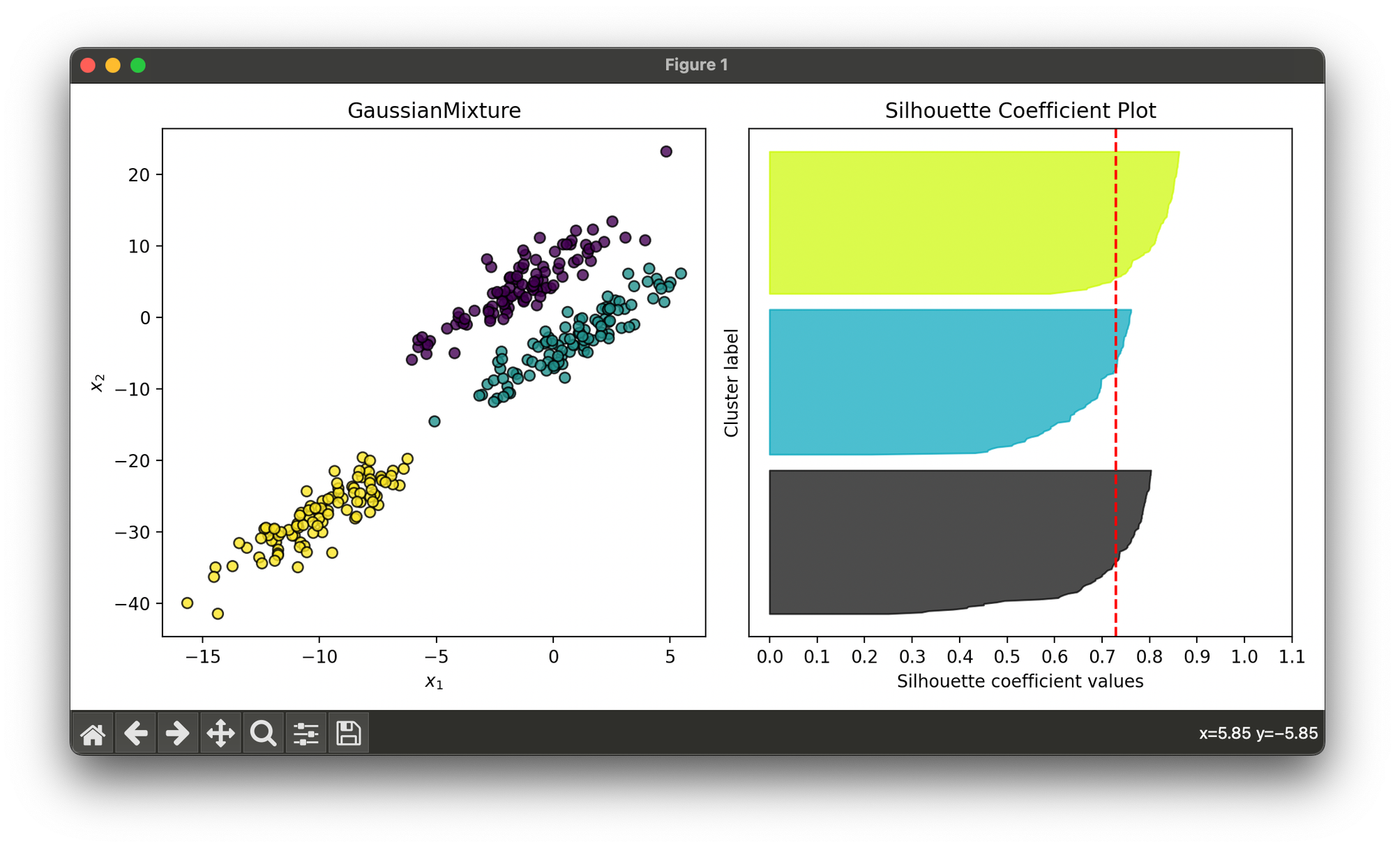
Test on synthesized dataset with 3 skewed Gaussian blobs:

from luma.clustering.mixture import GaussianMixture
from luma.visual.evaluation import ClusterPlot
from luma.metric.clustering import SilhouetteCoefficient

from sklearn.datasets import make_blobs
import matplotlib.pyplot as plt
import numpy as np

X, y = make_blobs(n_samples=300, 
                  centers=3, 
                  cluster_std=2.0, 
                  random_state=100)

trans_mat = np.array([[1, 2],
                      [0, 1]])

X_skew = X @ trans_mat

gmm = GaussianMixture(n_clusters=3, max_iter=100)
gmm.fit(X_skew)

fig = plt.figure(figsize=(10, 5))
ax1 = fig.add_subplot(1, 2, 1)
ax2 = fig.add_subplot(1, 2, 2)

clst = ClusterPlot(gmm, X_skew, cmap='viridis')
clst.plot(ax=ax1)

sil = SilhouetteCoefficient(X_skew, gmm.labels)
sil.plot(ax=ax2, show=True)

Applications

• Image Processing: GMMs are used in image segmentation, where each Gaussian distribution can model the color distribution of a different segment.
• Speech Recognition: In speech processing, GMMs can model the distribution of audio features for different phonemes or words.
• Anomaly Detection: By modeling normal behavior with a GMM, anomalies can be detected as data points that have low probability under the model.

Strengths and Limitations

Strengths

• Flexibility in Cluster Shape: GMM can accommodate clusters that are not spherical, as k-means does, due to its ability to model elliptical distributions.
• Soft Clustering: Provides the probability of membership in each cluster, allowing for more nuanced cluster assignments.
• Model Complexity Control: The covariance type (full, tied, diagonal, spherical) can be chosen to control the complexity of the model.

Limitations

• Sensitivity to Initialization: The final solution can be sensitive to the initial parameter values.
• Convergence to Local Maxima: The EM algorithm can converge to local maxima, leading to suboptimal solutions.
• Scalability: GMMs can be computationally intensive for large datasets or when modeling complex distributions with many components.

Advanced Topics

• Model Selection: Determining the optimal number of components in a GMM is a crucial task and can be approached using criteria such as the Bayesian Information Criterion (BIC) or the Akaike Information Criterion (AIC).
• Covariance Type Selection: Choosing the appropriate covariance structure (full, tied, diagonal, spherical) based on the dataset can significantly impact the model's performance.

References

1. Reynolds, Douglas A. "Gaussian mixture models." Encyclopedia of biometrics. Springer, Boston, MA, 2009. 659-663.
2. Bishop, Christopher M. "Pattern recognition and machine learning." Springer, 2006.