Multinomial Mixture Model (MMM)

Introduction

Multinomial Mixture Models are probabilistic models used for clustering categorical data. These models assume that the data are generated from a mixture of several multinomial distributions, each representing a cluster. The model is particularly useful in applications where objects are represented by counts or frequencies of events, such as text document clustering, where documents are represented by word counts.

Background and Theory

In contrast to Gaussian Mixture Models (GMMs) that are suited for continuous data, Multinomial Mixture Models are designed for discrete data. The key assumption is that the observed data are generated from a finite mixture of multinomial distributions, with each distribution corresponding to a different underlying process or cluster.

Mathematical Formulation

Given a dataset of $N$ items, where each item is a $D$-dimensional vector of counts, the probability of observing a particular item $x$ under a Multinomial Mixture Model is given by:

where:

• $K$ is the number of clusters (multinomial distributions) in the mixture.
• $\pi_k$ is the mixing coefficient for cluster $k$, indicating the probability that an item belongs to cluster $k$, with $\sum_{k=1}^{K} \pi_k = 1$.
• $\text{Mult}(x|p_k)$ is the probability of item $x$ under the multinomial distribution for cluster $k$, characterized by the parameter vector $p_k = (p_{k1}, p_{k2}, \cdots, p_{kD})$, where $p_{kj}$ is the probability of the $j$-th category in the $k$-th cluster, and $\sum_{j=1}^{D} p_{kj} = 1$.

Procedural Steps

Initialization

Choose the number of clusters $K$. Initialize the mixing coefficients $\pi_k$ and the probability vectors $p_k$ for each cluster.

Expectation (E) Step

Calculate the posterior probabilities (responsibilities) that each item belongs to each cluster, given the current parameters. For item $i$ and cluster $k$, this is:

Maximization (M) Step

Update the parameters $\pi_k$ and $p_k$ to maximize the expected log-likelihood of the observed data, given the current responsibilities:

• Update $\pi_k$:
  $\pi_k = \frac{1}{N} \sum_{i=1}^{N} \gamma_{ik}$
• Update $p_k$: For each category $j$ in cluster $k$, update $p_{kj}$:
  $p_{kj} = \frac{\sum_{i=1}^{N} \gamma_{ik} x_{ij}}{\sum_{j=1}^{D} \sum_{i=1}^{N} \gamma_{ik} x_{ij}}$

Iteration and Convergence

Repeat the E and M steps until the change in the log-likelihood or the parameters between iterations falls below a predefined threshold.

Implementation

Parameters

• n_clusters: int
  Number of clusters(mixtures) to estimate
  
• max_iter: int, default = 100
  Maximum amount of iteration
  
• tol: float, default = 0.00001
  Tolerance for early convergence
  

Examples

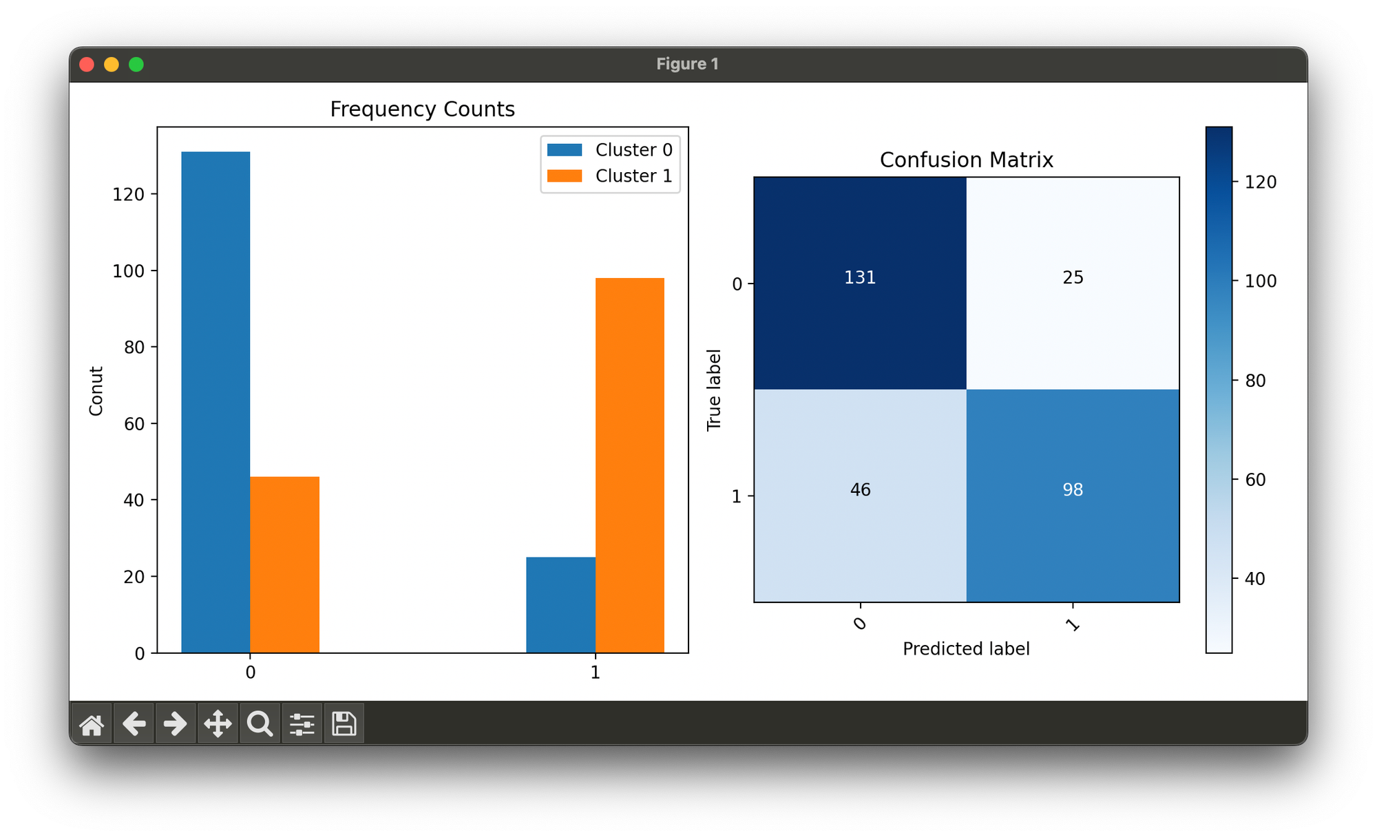
Test on synthesized 2D multinomial dataset with 2 mixtures:

from luma.clustering.mixture import MultinomialMixture
from luma.visual.evaluation import ConfusionMatrix

import matplotlib.pyplot as plt
import numpy as np


def generate_multi_dataset(n_samples: int, 
                           component_probs: list, 
                           mixture_weights: list) -> tuple:
    n_components = len(component_probs)
    dataset, labels = [], []
    for _ in range(n_samples):
        component = np.random.choice(range(n_components), p=mixture_weights)
        sample = np.random.multinomial(1, component_probs[component])
        
        dataset.append(sample)
        labels.append(component)
        
    return np.array(dataset), np.array(labels)


X, y = generate_multi_dataset(n_samples=300,
                              component_probs=[[0.2, 0.8],
                                               [0.7, 0.3]],
                              mixture_weights=[0.5, 0.5])

mmm = MultinomialMixture(n_clusters=2, max_iter=1000)
mmm.fit(X)

fig = plt.figure(figsize=(10, 5))
ax1 = fig.add_subplot(1, 2, 1)
ax2 = fig.add_subplot(1, 2, 2)

n_clusters = 2
bincounts = [np.bincount(X[y == i, 0]) for i in range(2)]

width = 0.2
ax1.bar(np.arange(n_clusters) - width / 2, bincounts[0], 
        width=width,
        label='Cluster 0')

ax1.bar(np.arange(n_clusters) + width / 2, bincounts[1], 
        width=width,
        label='Cluster 1')

ax1.set_xticks([0, 1])
ax1.set_ylabel('Conut')
ax1.set_title('Frequency Counts')
ax1.legend()

conf = ConfusionMatrix(y_true=y, y_pred=mmm.labels)
conf.plot(ax=ax2, show=True)

Applications

• Text Clustering: Grouping documents into topics based on word frequencies.
• Market Basket Analysis: Clustering customer purchase patterns to identify common baskets of products.
• Genetic Sequence Analysis: Clustering sequences into groups based on the frequency of nucleotides or amino acids.

Strengths and Limitations

Strengths

• Suitable for Categorical Data: Specifically designed to handle discrete count data efficiently.
• Interpretable Clusters: The parameters of the multinomial distributions can provide insights into the characteristics of each cluster.

Limitations

• Assumption of Independence: Assumes that the features (e.g., words in text clustering) are conditionally independent given the cluster, which may not always be true.
• Selection of Number of Clusters: Like other mixture models, determining the optimal number of clusters $K$ requires additional criteria or validation methods.

Advanced Topics

• Model Selection: Techniques like Bayesian Information Criterion (BIC) or Cross-Validation can be used to select the number of clusters.
• Extension to Other Distributions: For different types of data, the multinomial distribution can be replaced with other appropriate distributions within the mixture model framework.

References

1. McLachlan, Geoffrey, and Thriyambakam Krishnan. The EM algorithm and extensions. John Wiley & Sons, 2007.
2. Blei, David M., Andrew Y. Ng, and Michael I. Jordan. "Latent dirichlet allocation." Journal of machine Learning research 3.Jan (2003): 993-1022.