Normalized Spectral Clustering

Introduction

Normalized Spectral Clustering refines the standard Spectral Clustering approach by normalizing the data in a way that emphasizes the intrinsic geometry of the data space. This normalization step makes the algorithm more robust to changes in the data scale and improves its ability to identify clusters within complex datasets.

Background and Theory

The central idea behind Normalized Spectral Clustering is to use the spectrum (eigenvalues) of the normalized Laplacian matrix of a graph to perform dimensionality reduction before clustering. This process involves constructing a graph that represents the data, computing the normalized Laplacian matrix, and then using its eigenvalues and eigenvectors to find a low-dimensional representation of the data that highlights its cluster structure.

Mathematical Foundations

Given a dataset $X = \{x_1, x_2, \ldots, x_n\}$, we construct a weighted graph $G = (V, E)$, where each vertex $v_i \in V$ corresponds to a data point $x_i$, and each edge $(i, j) \in E$ is weighted by a similarity measure $W_{ij}$ between $x_i$ and $x_j$. The degree matrix $D$ is defined as before, and the normalized Laplacian matrix is used, which can be defined in two common forms:

1. Symmetric Normalized Laplacian:

   $L_{\text{sym}} = D^{-1/2} L D^{-1/2} = I - D^{-1/2} W D^{-1/2}$

2. Random Walk Normalized Laplacian:

   $L_{\text{rw}} = D^{-1} L = I - D^{-1} W$

Both forms of the normalized Laplacian are used to facilitate a clustering that respects the manifold structure of the data.

Procedural Steps

1. Similarity Graph Construction: Construct a similarity graph $G$ by calculating the pairwise similarities $W_{ij}$ between points in $X$.
2. Compute the Normalized Laplacian: Calculate the degree matrix $D$ and then compute the normalized Laplacian matrix $L_{\text{sym}}$ or $L_{\text{rw}}$.
3. Eigenvalue Decomposition: Perform eigenvalue decomposition on the normalized Laplacian to obtain its eigenvalues $\lambda_1, \lambda_2, \ldots, \lambda_n$ and corresponding eigenvectors $u_1, u_2, \ldots, u_n$.
4. Map to Lower-Dimensional Space: Form a feature vector matrix $U \in \mathbb{R}^{n \times k}$ from the $k$ eigenvectors corresponding to the $k$ smallest non-zero eigenvalues. Normalize the rows of $U$ to have unit length.
5. Clustering in Reduced Space: Apply a clustering algorithm like K-means on the rows of $U$ to identify clusters.

Mathematical Formulations

The choice between $L_{\text{sym}}$ and $L_{\text{rw}}$ affects the subsequent steps. For $L_{\text{sym}}$, the row normalization of $U$ ensures that data points are mapped to the surface of a unit hypersphere in the reduced space, making them amenable to clustering by methods like K-means.

The eigenvalue problem for the symmetric normalized Laplacian is:

For the random walk Laplacian, the problem becomes:

where $u$ are the eigenvectors, and $\lambda$ are the corresponding eigenvalues.

Implementation

Parameters

• n_clusters: int
  Number of clusters to estimate
  
• gamma: float, default = 1.0
  Scaling factor for Gaussian(RBF) kernel
  
• strategy: Literal['symmetric', 'random-walk'], default = ‘symmetric’
  Normalization strategy
  

Examples

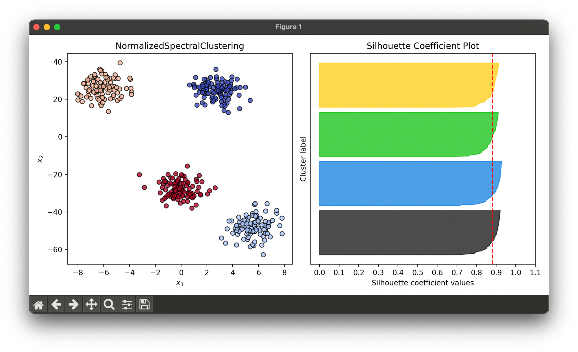
Test on synthesized data with differently scaled 4 blobs:

from luma.clustering.spectral import NormalizedSpectralClustering
from luma.metric.clustering import SilhouetteCoefficient
from luma.visual.evaluation import ClusterPlot

from sklearn.datasets import make_blobs
import matplotlib.pyplot as plt

X, y = make_blobs(n_samples=400, 
                  centers=4, 
                  cluster_std=1.0, 
                  random_state=10)

X[:, 1] *= 5

nsp = NormalizedSpectralClustering(n_clusters=4, 
                                   gamma=1.0, 
                                   strategy='symmetric')

nsp.fit(X)

fig = plt.figure(figsize=(10, 5))
ax1 = fig.add_subplot(1, 2, 1)
ax2 = fig.add_subplot(1, 2, 2)

clst = ClusterPlot(nsp, X, cmap='coolwarm')
clst.plot(ax=ax1)

sil = SilhouetteCoefficient(X, nsp.labels)
sil.plot(ax=ax2, show=True)

Applications

• Community Detection in Networks: Identifying natural communities within large social or information networks.
• Image Segmentation: Grouping pixels into segments representing different objects or regions.
• Biological Data Analysis: Clustering genes or proteins with similar expression patterns or functions.

Strengths and Limitations

Strengths

• Effective in identifying clusters with non-linear boundaries.
• Robust to variations in data scale and density.

Limitations

• Computationally intensive, especially for large datasets.
• Performance depends on the choice of the similarity graph and its parameters.

Advanced Topics

• Scalability Improvements: Techniques like sparse matrix representations and approximate eigendecomposition methods to handle large-scale datasets.
• Multiscale Spectral Clustering: Adapting the algorithm to reveal hierarchical structure by varying the resolution of the clustering.

References

1. Von Luxburg, Ulrike. "A tutorial on spectral clustering." Statistics and computing 17, no. 4 (2007): 395-416.
2. Shi, Jianbo, and Jitendra Malik. "Normalized cuts and image segmentation." IEEE Transactions on pattern analysis and machine intelligence 22, no. 8 (2000): 888-905.