Spectral Clustering

Introduction

Spectral Clustering is a versatile algorithm for grouping objects in various applications, such as image and social network segmentation. Unlike traditional clustering methods like K-means, Spectral Clustering doesn't make strong assumptions about the form of the clusters. It can identify clusters with irregular boundaries by using the eigenvalues (spectrum) of similarity matrices, hence the name "Spectral Clustering".

Background and Theory

Spectral Clustering is based on graph theory. The fundamental idea is to model the data as a graph, where each data point represents a node, and the edge between two nodes represents the similarity between those two points. The goal is to partition this graph into subgraphs (clusters) such that the edges between different groups have low weights (low similarity) and the edges within a group have high weights (high similarity).

Mathematical Foundations

Given a set of data points, $X = \{x_1, x_2, \ldots, x_n\}$, we construct a similarity graph $G = (V, E)$, where $V$ is a set of vertices corresponding to the data points, and $E$ is a set of edges connecting the vertices. The weight of an edge $(i, j) \in E$, denoted by $W_{ij}$, measures the similarity between $x_i$ and $x_j$. A common choice for $W_{ij}$ is the Gaussian similarity function:

where $\sigma$ is a free parameter that controls the width of the neighborhoods.

The degree of a vertex $i$, denoted by $D_i$, is defined as the sum of the weights of all edges connected to it:

The degree matrix $D$ is a diagonal matrix with the degrees $D_1, D_2, \ldots, D_n$ on its diagonal.

The Laplacian matrix $L$ is defined as $L = D - W$. It plays a crucial role in Spectral Clustering. There are several variants of the Laplacian matrix; the most commonly used is the normalized Laplacian, defined as:

where $I$ is the identity matrix.

Procedural Steps

1. Construct the similarity graph: Decide on a graph structure (e.g., $k$-nearest neighbors or $\epsilon$-neighborhoods) and construct the graph by computing the edge weights using a similarity measure.
2. Compute the Laplacian matrix: Calculate the degree matrix $D$ and the Laplacian matrix $L$ based on the similarity graph.
3. Eigenvalue decomposition: Perform eigenvalue decomposition on the Laplacian matrix to obtain its eigenvalues and eigenvectors.
4. Map each point to a lower-dimensional representation: Select the $k$ smallest eigenvalues and their corresponding eigenvectors. Form a matrix $U \in \mathbb{R}^{n \times k}$ with these eigenvectors as columns. Then, normalize the rows of $U$ to have unit length.
5. Cluster the points in the new space: Use a standard clustering algorithm, like K-means, on the rows of $U$ to cluster the data points.

Implementation

Parameters

• n_clusters: int
  Number of clusters to estimate
  
• gamma: float, default = 1.0
  Scaling factor for Gaussian(RBF) kernel
  

Examples

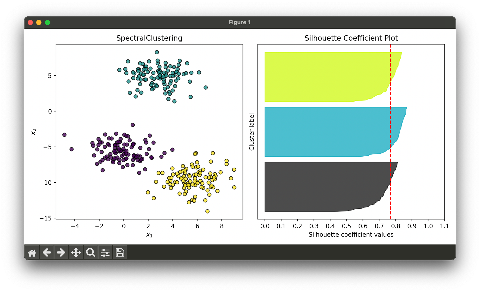
Test on synthesized dataset with 3 blobs:

from luma.clustering.spectral import SpectralClustering
from luma.metric.clustering import SilhouetteCoefficient
from luma.visual.evaluation import ClusterPlot

from sklearn.datasets import make_blobs
import matplotlib.pyplot as plt

X, y = make_blobs(n_samples=300, 
                  centers=3, 
                  cluster_std=1.5, 
                  random_state=10)

sp = SpectralClustering(n_clusters=3, gamma=1.0)
sp.fit(X)

fig = plt.figure(figsize=(10, 5))
ax1 = fig.add_subplot(1, 2, 1)
ax2 = fig.add_subplot(1, 2, 2)

clst = ClusterPlot(sp, X, cmap='viridis')
clst.plot(ax=ax1)

sil = SilhouetteCoefficient(X, sp.labels)
sil.plot(ax=ax2, show=True)

Applications

• Image segmentation: Partitioning an image into segments with similar textures or colors.
• Social network analysis: Identifying communities within social networks based on the pattern of connections.
• Dimensionality reduction: When used in conjunction with other algorithms, it can help to reveal the structure at different scales.

Strengths and Limitations

Strengths

• Capable of detecting complex cluster structures.
• Does not assume spherical clusters, unlike K-means.
• Works well for small to medium-sized datasets.

Limitations

• Selection of parameters (e.g., the number of clusters and the choice of similarity measure) can significantly affect the results.
• Computationally expensive for large datasets, especially due to the eigenvalue decomposition step.
• The algorithm's performance is highly sensitive to the choice of the graph construction method.

Advanced Topics

• Kernelized Spectral Clustering: Extends Spectral Clustering to nonlinearly separable datasets by applying the kernel trick.
• Large-scale Spectral Clustering: Techniques such as Nyström approximation and landmark-based spectral clustering have been developed to handle large datasets more efficiently.

References

1. Ulrike von Luxburg, "A Tutorial on Spectral Clustering," Statistics and Computing 17, no. 4 (2007): 395-416.
2. Andrew Y. Ng, Michael I. Jordan, and Yair Weiss, "On Spectral Clustering: Analysis and an algorithm," Advances in Neural Information Processing Systems 14 (2001).