OPTICS

Introduction

The OPTICS (Ordering Points To Identify the Clustering Structure) algorithm, introduced by Mihael Ankerst, Markus M. Breunig, Hans-Peter Kriegel, and Jörg Sander in 1999, extends the concepts of the DBSCAN (Density-Based Spatial Clustering of Applications with Noise) algorithm. It addresses one of DBSCAN's main limitations: the difficulty of identifying clusters of varying density. OPTICS does not explicitly produce clusters; instead, it creates an augmented ordering of the database representing its density-based clustering structure. This ordering allows for the extraction of clusters with varying densities by analyzing the generated reachability plot.

Background and Theory

OPTICS organizes data points in a manner that spatially close points become neighbors in the ordering, preserving the density-based clustering structure. It introduces two key concepts: core distance and reachability distance, which are crucial for understanding the density relationship between points.

Mathematical Foundations

Given a dataset $D$ consisting of points in a metric space, the OPTICS algorithm relies on two parameters:

• $\epsilon$: Maximum radius to consider for the neighborhood of a point.
• $MinPts$: Minimum number of points required to form a dense region (similar to DBSCAN).

Core Distance

For a point $p$ in $D$, the core distance is defined as the smallest distance $\epsilon'$ such that there are at least $MinPts$ points within $\epsilon'$ of $p$, including $p$ itself. Mathematically, it is expressed as:

where $N_{\epsilon}(p)$ denotes the $\epsilon$-neighborhood of $p$, and $d(p, O_{MinPts})$ is the distance from $p$ to its $MinPts$-th nearest neighbor.

Reachability Distance

The reachability distance of a point $p$ from point $o$ is defined as the maximum of the core distance of $o$ and the Euclidean distance $d(o, p)$, ensuring that the reachability distance respects the minimum density criterion specified by $MinPts$. It is defined as:

OPTICS Algorithm

The OPTICS algorithm processes each point in the dataset, computing its core distance and updating the reachability distance for its neighbors. The main steps are as follows:

1. Initialization: Create an empty ordered list representing the clustering structure.
2. Process Each Point:
   • For a point $p$ not yet processed, retrieve its $\epsilon$-neighborhood.
   • Calculate $p$'s core distance.
   • Insert $p$ into the ordered list, and if $p$ is a core point, update the reachability distances of its neighbors.
   • Use a priority queue to determine the next point to process based on the smallest reachability distance.

Generating Clusters from Reachability Plot

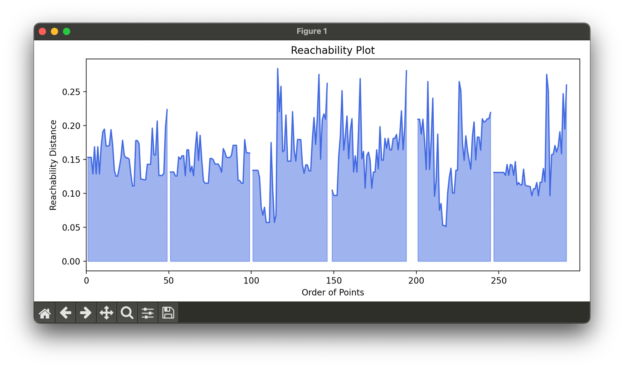
A reachability plot is derived from the ordered list, where each point's reachability distance is plotted. Clusters can be extracted by identifying valleys in the reachability plot, which correspond to regions of high density.

Implementation

Parameters

• epsilon: float, default = 1.0
  Radius of neighborhood hypersphere
  
• min_points: int, default = 5
  Minimum nuber of points to form a cluster
  
• threshold: float, default = 1.5
  Threshold for filtering samples with large reachabilities
  

Examples

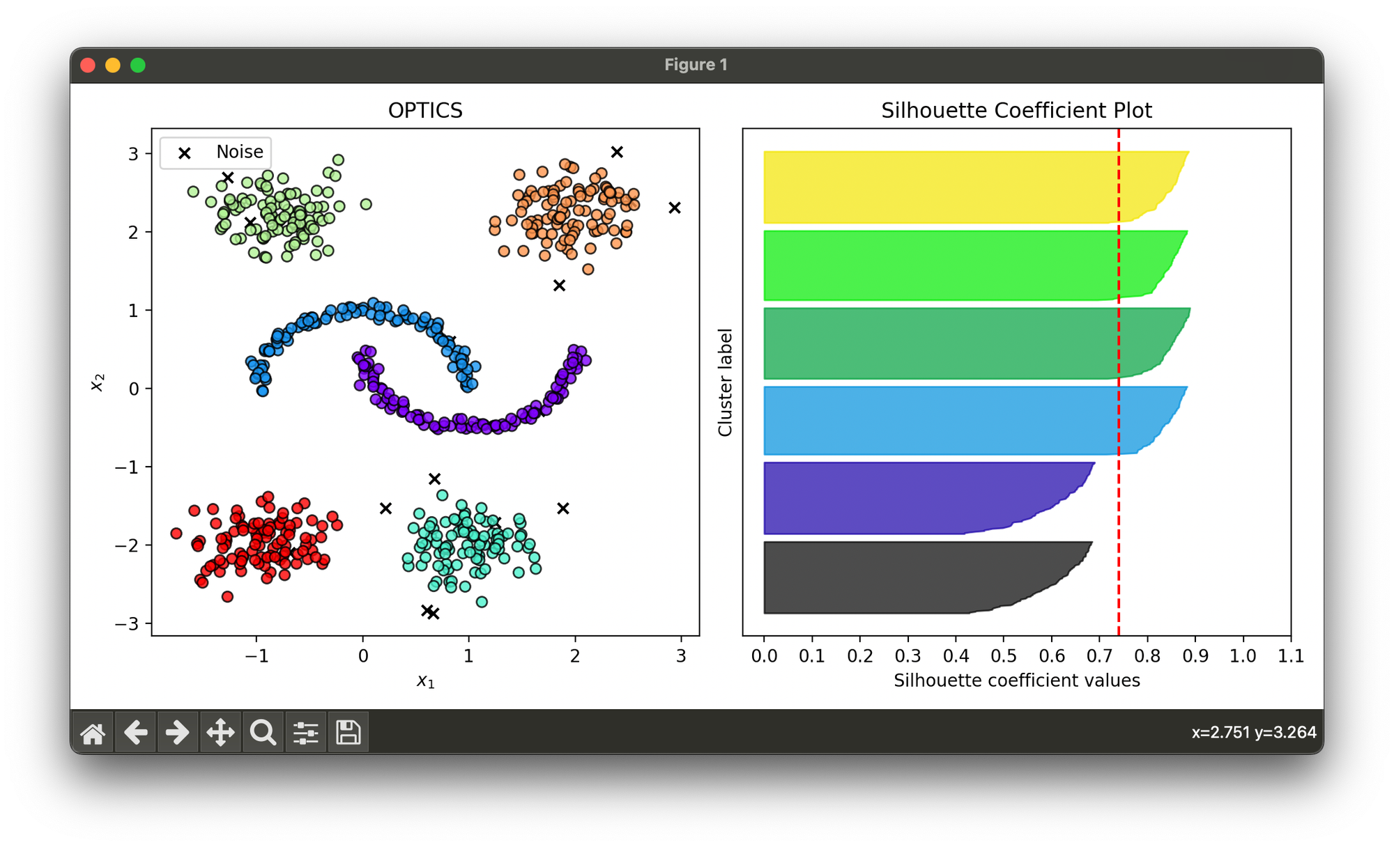
Test on synthesized dataset comprised of blobs and moons datasets:

from luma.clustering.density import OPTICS
from luma.visual.evaluation import ClusterPlot
from luma.metric.clustering import SilhouetteCoefficient

from sklearn.datasets import make_blobs, make_moons
import matplotlib.pyplot as plt
import numpy as np


num = 100
moons, _ = make_moons(n_samples=num, noise=0.05)

blobs, _ = make_blobs(n_samples=num, 
                      centers=[(-0.75,2.25), (1.0, -2.0)], 
                      cluster_std=0.3)

blobs2, _ = make_blobs(n_samples=num, 
                       centers=[(2,2.25), (-1, -2.0)], 
                       cluster_std=0.3)

X = np.vstack([moons, blobs, blobs2])

opt = OPTICS(epsilon=0.3,
             min_points=5,
             threshold=1.5)

opt.fit(X)
opt.plot_reachability()

fig = plt.figure(figsize=(10, 5))
ax1 = fig.add_subplot(1, 2, 1)
ax2 = fig.add_subplot(1, 2, 2)

clst = ClusterPlot(opt, X)
clst.plot(ax=ax1)

sil = SilhouetteCoefficient(X, opt.labels)
sil.plot(ax=ax2, show=True)

Applications

OPTICS is versatile and can be applied across various domains where clustering of spatial data is required:

• Geographic Information Systems (GIS): Analyzing spatial patterns, such as identifying regions of similar land use.
• Astronomy: Grouping stars or galaxies based on spatial features.
• Market Research: Segmenting customers based on purchasing behavior and geographical location.

Strengths and Limitations

Strengths

• Flexibility in Cluster Density: Capable of identifying clusters with different densities, which is a significant advantage over DBSCAN.
• Robustness to Noise: Similar to DBSCAN, OPTICS is effective in handling noise and outliers in the dataset.
• No Need for $MinPts$ Specification: While $MinPts$ is used, its selection is less critical compared to $\epsilon$ in DBSCAN, as OPTICS processes data with a range of $\epsilon$ values.

Limitations

• Complexity: The algorithm is computationally more complex than DBSCAN, making it slower for large datasets.
• Parameter Sensitivity: The quality of the clustering result still depends on the choice of parameters, although to a lesser extent than in DBSCAN.
• Interpretation of Results: The reachability plot, while informative, can sometimes be difficult to interpret, requiring experience to identify clusters accurately.

Advanced Topics

Scalability and Efficiency

Improving the efficiency of OPTICS for large datasets involves optimizing the data structure used for managing points and their reachability distances. Techniques such as spatial indexing (e.g., R-trees) and parallel processing can significantly reduce computational overhead.

Variants of OPTICS

Several variants of OPTICS have been developed to address specific challenges, such as handling high-dimensional data or improving computational efficiency. These include OPTICS-OF for outlier detection and HiCO for hierarchical clustering in high-dimensional spaces.

Conclusion

OPTICS offers a flexible and powerful approach to clustering, capable of uncovering complex structures in data. Despite its computational complexity, its ability to deal with varying densities and noise makes it a valuable tool in the data scientist's toolkit.

References

1. Ankerst, Mihael, et al. "OPTICS: Ordering points to identify the clustering structure." ACM Sigmod Record 28.2 (1999): 49-60.
2. Kriegel, Hans-Peter, Peer Kröger, and Arthur Zimek. "Clustering high-dimensional data: A survey on subspace clustering, pattern-based clustering, and correlation clustering." ACM Transactions on Knowledge Discovery from Data (TKDD) 3.1 (2009): 1-58.