Convolution Layer

Introduction

The convolution operation is a cornerstone in many fields such as signal processing, image processing, and machine learning. It involves the integration of two functions, showing how the shape of one is modified by the other. The Fast Fourier Transform (FFT) provides an efficient way to compute convolutions, especially when dealing with large datasets or real-time processing, where traditional convolution becomes computationally expensive.

Background and Theory

Convolution

Mathematically, convolution is defined for two functions $f(t)$ and $g(t)$ as:

In discrete terms, for sequences $f[n]$ and $g[n]$ of length $N$, the convolution is given by:

where $n-m$ is evaluated modulo $N$ in the case of circular convolution.

Fourier Transform

The Fourier Transform (FT) of a continuous signal $x(t)$ is defined as:

For discrete signals, the Discrete Fourier Transform (DFT) is used:

The DFT transforms a signal from the time domain into the frequency domain.

The Convolution Theorem

The Convolution Theorem states that the Fourier Transform of the convolution of two signals is the pointwise product of their Fourier Transforms:

This theorem forms the basis for using FFT to compute convolutions efficiently.

Procedural Steps

1. Padding the Signals: To ensure the output is not affected by circular convolution effects, the sequences $f[n]$ and $g[n]$ are padded with zeros to at least the length $N + M - 1$, where $N$ and $M$ are the lengths of the original sequences.
2. Applying FFT: Compute the FFT of the padded sequences, $\hat{f}$ and $\hat{g}$.
3. Pointwise Multiplication: Multiply the results of the FFTs element-wise.
4. Inverse FFT: Apply the inverse FFT to the product to get the result in the time domain, which is the convolution of $f[n]$ and $g[n]$.
5. Trimming: Trim the result to remove the extra padding, if necessary.

Mathematical Formulation

Given two sequences $f[n]$ and $g[n]$, their FFTs are computed as follows:

After zero-padding $f[n]$ and $g[n]$ to the same length $P \geq N + M - 1$, their FFTs are:

The convolution result in the frequency domain is:

Applying the inverse FFT:

Tensor Convolution Accelerated by FFT

Tensor convolution is an extension of traditional convolution techniques, applied particularly in fields like computer vision and deep learning, where multidimensional data structures known as tensors are manipulated. The Fast Fourier Transform (FFT) accelerates tensor convolution significantly, enhancing the efficiency of operations such as those in convolutional neural networks (CNNs). Below, we delve into the theory, procedure, and specific considerations for implementing tensor convolution using FFT.

FFT for Tensors

FFT can be extended to multidimensional data to speed up the convolution operation in multiple dimensions simultaneously. The key principle remains utilizing the Convolution Theorem, which states that convolution in the spatial domain corresponds to element-wise multiplication in the frequency domain. For tensors, this principle applies in each dimension independently.

3D Tensor Convolution

Consider a 3D input tensor $X$ and a kernel $K$, both extended to the same size with zero-padding to avoid circular convolution artifacts. Let their sizes after padding be $P \times Q \times R$.

The FFT-based convolution can be computed as follows:

1. FFT Computation: Compute the FFT of both tensors $X$ and $K$ across all three dimensions:

   $\hat{X}[u, v, w] = \sum_{x=0}^{P-1} \sum_{y=0}^{Q-1} \sum_{z=0}^{R-1} X[x, y, z] \exp\left[{-j 2\pi \left(\frac{ux}{P} + \frac{vy}{Q} + \frac{wz}{R}\right)}\right]$
   $\hat{K}[u, v, w] = \sum_{x=0}^{P-1} \sum_{y=0}^{Q-1} \sum_{z=0}^{R-1} K[x, y, z] \exp\left[{-j 2\pi \left(\frac{ux}{P} + \frac{vy}{Q} + \frac{wz}{R}\right)}\right]$

2. Element-wise Multiplication: Multiply the Fourier transforms $\hat{X}$ and $\hat{K}$ element-wise.

3. Inverse FFT: Apply the inverse FFT to obtain the convolved tensor in the spatial domain:

   $Y[x, y, z] = \text{IFFT}(\hat{X} \odot \hat{K})[x, y, z]$

   Here, $Y[x, y, z]$ represents the output tensor, which is the result of convolving $X$ with $K$.

Implementation

Parameters

• in_channels: int
  Number of input channels
  
• out_channels: int
  Number of output channels(filters)
  
• filter_size: int
  Size of each filter
  
• stride: int
  Step size for filters during convolution
  
• padding: Literal['same', 'valid'], default = ‘sam
  Padding stratagies (valid for no padding, same for typical 0-padding)
  
• activation: FuncType, default = ‘relu’
  Type of activation function
  
• initializer: InitType, default = ‘auto’
  Type of weight initializer
  
• optimizer: Optimizer, default = None
  Optimizer for weight update
  
• lambda_: float, default = 0.0
  L2-regularization strength
  

Examples

from luma.preprocessing.scaler import StandardScaler
from luma.preprocessing.encoder import OneHotEncoder
from luma.model_selection.split import TrainTestSplit, BatchGenerator
from luma.metric.classification import Accuracy

from luma.neural.layer import Convolution, Flatten, Dense, Sequential
from luma.neural.loss import SoftmaxLoss
from luma.neural.optimizer import AdamOptimizer

from sklearn.datasets import load_digits
import matplotlib.pyplot as plt
import numpy as np

X, y = load_digits(return_X_y=True)

sc = StandardScaler()
X_sc = sc.fit_transform(X)

X_train, X_test, y_train, y_test = TrainTestSplit(
    X_sc, y, test_size=0.3, shuffle=True, stratify=True
).get

en = OneHotEncoder()
y_train = en.fit_transform(y_train.reshape(-1, 1))
y_test = en.fit_transform(y_test.reshape(-1, 1))

X_train = X_train.reshape(-1, 1, 8, 8)
X_test = X_test.reshape(-1, 1, 8, 8)

epochs = 30
batch_size = 100

# -----------------------------------------------------------#
model = Sequential(
    Convolution(1, 6, 5, padding="same", activation="relu"),
    Convolution(6, 12, 5, padding="same", activation="relu"),
    Flatten(),
    Dense(768, 10, activation=None),
)

model.set_optimizer(AdamOptimizer(), learning_rate=0.001)
model.set_loss(SoftmaxLoss())
print(repr(model))
# -----------------------------------------------------------#

losses = []
for i in range(1, epochs + 1):
    epoch_loss = []
    for j, (X_batch, y_batch) in enumerate(
        BatchGenerator(X_train, y_train, batch_size=batch_size), start=1
    ):
        loss = model(X_batch, y_batch, is_train=True)
        losses.append(loss)
        epoch_loss.append(loss)

    print(f"Epoch {i}/{epochs} - Avg. Loss: {np.average(epoch_loss)}")

test_out = model.forward(X_test)
score = Accuracy.score(y_test.argmax(axis=1), test_out.argmax(axis=1))

r_id = np.random.choice(range(len(X_test)), 1)[0]

X_sample = X_test[r_id][np.newaxis]
first_out = model[0][1].forward(X_sample)
second_out = model[1][1].forward(first_out)

outs = np.vstack((first_out.squeeze(), second_out.squeeze()))

plt.figure(figsize=(10, 5))
plt.suptitle(
    f"Convolution Result for Digit '{y_test[r_id].argmax()}' "
    + f"[Acc: {score * 100:.2f} %]"
)

rows, cols = 3, 6
for i in range(1, 19):
    ax = plt.subplot(rows, cols, i)
    ax.imshow(
        outs[i - 1],
        cmap="Blues",
        interpolation="bilinear",
    )
    ax.set_xticks([])
    ax.set_yticks([])
    ax.set_title(f"Filter {i}")

plt.tight_layout()
plt.show()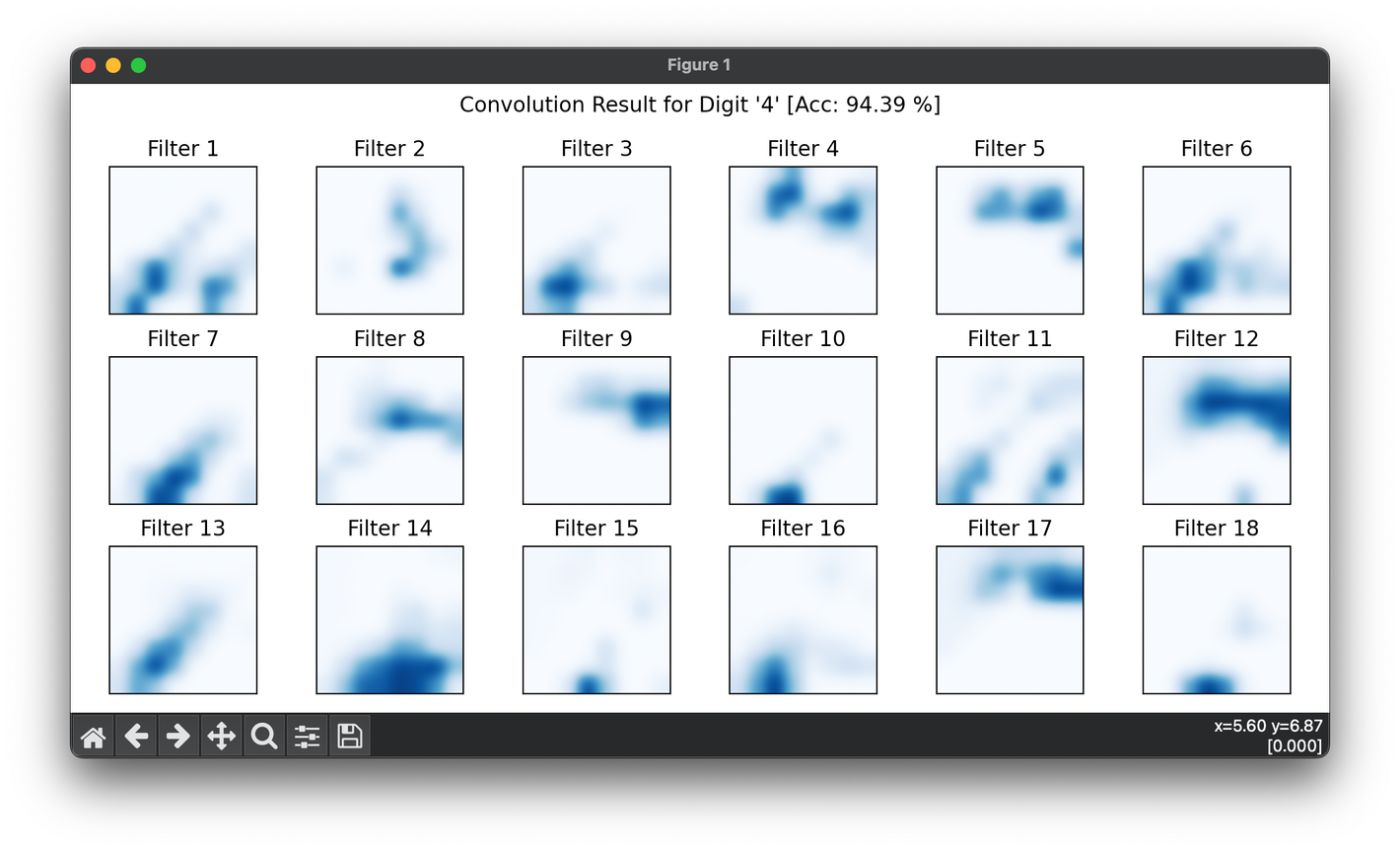

Applications

The FFT-based convolution is widely used in:

• Digital Signal Processing: For filtering signals in time-domain using frequency-domain multiplication.
• Image Processing: In operations like blurring, sharpening, and edge detection.
• Deep Learning: Particularly in convolutional neural networks where convolution operations are fundamental.

Discussion on Strengths and Limitations

Strengths

• Efficiency: FFT reduces the computational complexity of convolution from $O(N^2)$ to $O(N \log N)$.
• Scalability: FFT-based convolution is highly effective for large data sets typical in real-time systems.

Limitations

• Circular Convolution: The need for careful padding to avoid artifacts due to the circular nature of FFT-based convolution.
• Overhead: FFT and IFFT introduce computational overhead, particularly noticeable with smaller data sets or when the efficiency gain from reduced complexity is minimal.

Advanced Topics

• Multi-dimensional FFT: Extending the convolution via FFT to two or more dimensions, applicable in areas such as volumetric data processing and multi-channel systems.
• Optimization Techniques: Various algorithms and hardware implementations that optimize FFT computation, such as the split-radix FFT and hardware acceleration through GPUs.

Conclusion

Convolution via FFT is a powerful technique that leverages the efficiency of the Fourier Transform to perform convolutions in an optimized manner. The understanding and application of this method across various domains illustrate its fundamental importance in modern computational techniques.

References

1. Smith, Steven W. "The Scientist and Engineer's Guide to Digital Signal Processing." California Technical Publishing, 1997.
2. Brigham, E. Oran. "The Fast Fourier Transform and Its Applications." Prentice Hall, 1988.