Dense Layer

Introduction

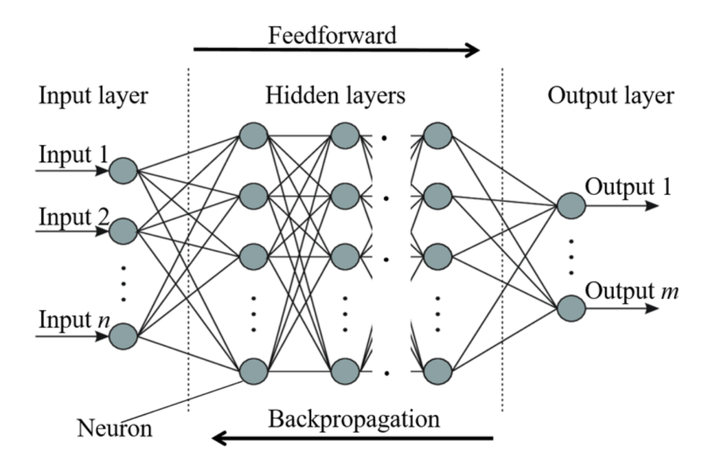
The dense layer, or fully connected layer, is an essential building block in many neural network architectures used for a broad range of machine learning tasks. These layers are characterized by their fully connected nature, where each input is connected to every output via a set of learnable weights and biases. Understanding how backpropagation works in dense layers is critical for optimizing neural network training, as it allows for the efficient adjustment of these parameters based on the loss gradient.

Background and Theory

Dense Layer Structure

A dense layer transforms its input through a linear combination followed by a nonlinear activation function. Mathematically, the output $\mathbf{y}$ of a dense layer given an input vector $\mathbf{x}$ is:

where:

• $\mathbf{W}$ is the weight matrix,
• $\mathbf{b}$ is the bias vector,
• $\sigma$ is the nonlinear activation function.

Backpropagation Overview

Backpropagation is a method used to compute the gradient of the loss function of a neural network with respect to its weights and biases. It involves two main phases:

1. Forward Pass: Compute the output of the network, layer by layer, using the input data.
2. Backward Pass: Propagate the error back through the network to compute the gradients.

Mathematical Formulation

Forward Pass

During the forward pass, each neuron in the dense layer receives an input, applies a weighted sum with its weights and bias, and then passes the result through an activation function. The output $\mathbf{y}$ of the dense layer is computed as mentioned previously.

Backward Pass (Backpropagation)

The backward pass involves calculating the gradients of the loss function with respect to each parameter (weights and biases).

Let $L$ denote the loss function of the network. The gradients are calculated as follows:

Gradient w.r.t. Weights

The gradient of the loss $L$ with respect to the weight matrix $\mathbf{W}$ is given by:

Using the chain rule, the derivative $\frac{\partial \mathbf{y}}{\partial \mathbf{W}}$ can be computed, where $\frac{\partial L}{\partial \mathbf{y}}$ is the gradient of the loss with respect to the output of the layer, and $\mathbf{x}$ is the input to the layer.

Therefore:

Gradient w.r.t. Biases

Similarly, the gradient of the loss with respect to the bias vector $\mathbf{b}$ is:

Since the derivative of $\mathbf{y}$ with respect to $\mathbf{b}$ is the derivative of the activation function:

Update Rule

The weights and biases are updated using the gradients calculated during backpropagation, typically with an update rule such as:

where $\eta$ is the learning rate.

Implementation

Parameters

• in_features: int
  Number of input features
  
• out_features: int
  Number of output features
  
• activation: FuncType, default = ‘relu’
  Activation function
  
• initializer: InitType, default = ‘auto’
  Type of weight initializer
  
• optimizer: Optimizer, default = None
  Optimizer for weight update
  
• lambda_: float, default = 0.0
  L2-regularization strength
  

Applications

• Image Recognition: Dense layers aggregate learned features from convolutional layers to classify images.
• Natural Language Processing: Used in neural networks to interpret and make predictions based on textual data.
• Regression Tasks: Predict continuous variables using patterns learned from data.

Strengths and Limitations

Strengths

• Universal Approximation: Capable of approximating any continuous function given sufficient neurons and layers.
• Simplicity: Straightforward implementation and integration into various architectures.

Limitations

• Computationally Intensive: Requires a lot of computational power for large networks.
• Prone to Overfitting: Especially in networks with a large

number of parameters relative to the amount of training data.

Advanced Topics

Optimization Enhancements

Improving backpropagation includes techniques like momentum, RMSprop, and Adam, which help in converging faster and more reliably than standard stochastic gradient descent.

Regularization Techniques

Methods like dropout, L1/L2 regularization, and early stopping are crucial for preventing overfitting and improving the generalization of dense layers in large networks.

References

1. Goodfellow, Ian, et al. "Deep Learning." MIT press, 2016.
2. LeCun, Yann, Yoshua Bengio, and Geoffrey Hinton. "Deep learning." Nature 521.7553 (2015): 436-444.