
📌 사용 환경
Python 3.10.2
conda 24.9.0
JupyterLab 4.2.5
1. 다중 선형 회귀(Multiple Linear Regression)
나라별 기대 수명 예측
https://www.kaggle.com/datasets/kumarajarshi/life-expectancy-who
그러면 지금까지 X값이 하나인 단일 선형 회귀만 했는데, 다중 선형회귀도 크게 다를 건 없다.
X값이 많아지는거 뿐이다.
y = wx1 + wx2 + wx3 + ... + b 이렇게 된다.
그런데 이를 선으로 그을 수는 없다.
컴퓨터상에 그릴 수 있는 것은 오직 2차원까지다.
참고로 딥러닝에 가면 y = w1x1 + w1x2 + w1x3 + ... + w2x1 + w2x2 + ... + b 이렇게 된다.
그러면 실제 데이터처럼 X가 많으면 어떻게할까?
DataFrame으로 담으면 된다.
이번에는 캐글에 있는 데이터인 나라별 기대 수명을 예측하는 데이터다.
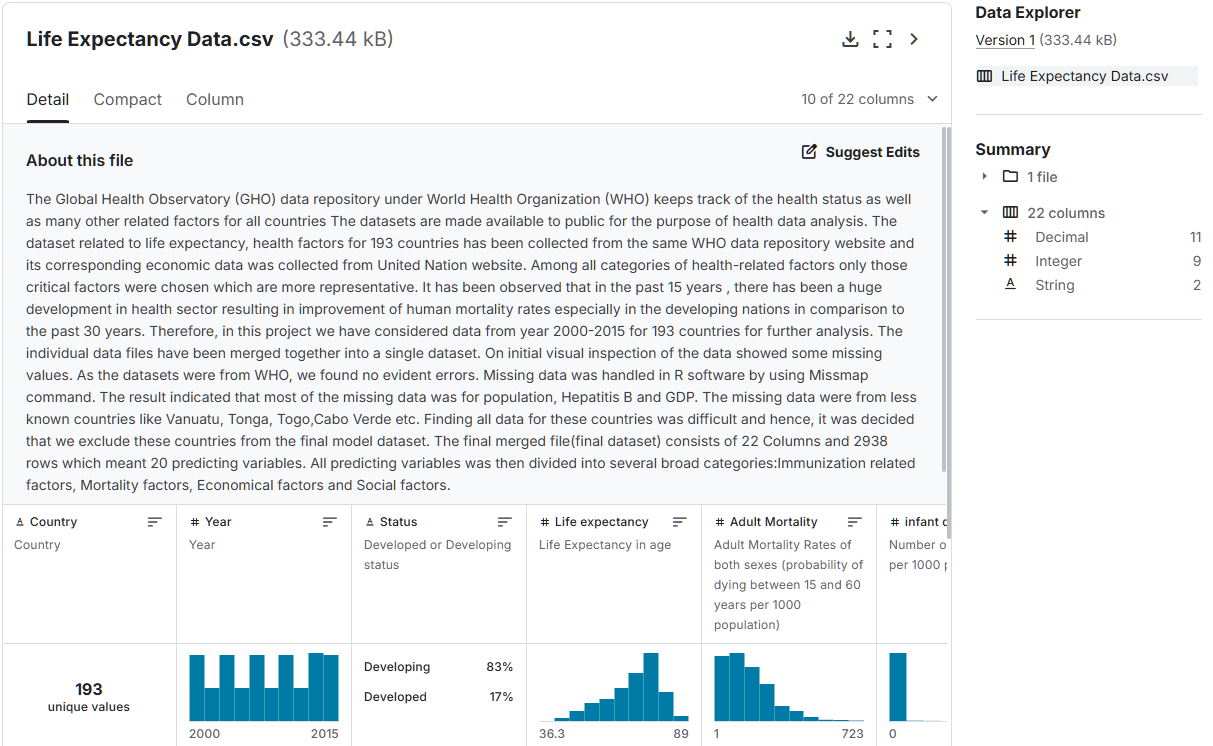
22개의 열로 target을 제외하면 wx1 + wx2 + ... wx20 + b가 될 것이다.
그런데 이중 몇개만 골라서 진행한다.
우선 필요한 라이브러리를 import하자.
import numpy as np
import pandas as pd
import seaborn as sns

import matplotlib.pyplot as plt
import matplotlib as mpl
mpl.rc("font", family="Malgun Gothic")
plt.rcParams["axes.unicode_minus"]=False

from sklearn.model_selection import train_test_split

from sklearn.linear_model import LinearRegression
from sklearn.metrics import mean_squared_error, mean_absolute_error
1.1. 데이터 전처리
데이터를 가져와서 전처리를 진행한다.
life=pd.read_csv("./data/life_expectancy.csv")
life.shape     # (2938, 22)
life.head()| Country | Year | Status | Life expectancy | Adult mortality | Infant deaths | Alcohol | Percentage expenditure | Hepatitis B | Measles | ... | Polio | Total expenditure | Diphtheria | HIV/AIDS | GDP | Population | Thinness 1-19 years | Thinness 5-9 years | Income composition of resources | Schooling | |
|---|---|---|---|---|---|---|---|---|---|---|---|---|---|---|---|---|---|---|---|---|---|
| 0 | Afghanistan | 2015 | Developing | 65.0 | 263.0 | 62 | 0.01 | 71.279624 | 65.0 | 1154 | ... | 6.0 | 8.16 | 65.0 | 0.1 | 584.259210 | 33736494.0 | 17.2 | 17.3 | 0.479 | 10.1 |
| 1 | Afghanistan | 2014 | Developing | 59.9 | 271.0 | 64 | 0.01 | 73.523582 | 62.0 | 492 | ... | 58.0 | 8.18 | 62.0 | 0.1 | 612.696514 | 327582.0 | 17.5 | 17.5 | 0.476 | 10.0 |
| 2 | Afghanistan | 2013 | Developing | 59.9 | 268.0 | 66 | 0.01 | 73.219243 | 64.0 | 430 | ... | 62.0 | 8.13 | 64.0 | 0.1 | 631.744976 | 31731688.0 | 17.7 | 17.7 | 0.470 | 9.9 |
| 3 | Afghanistan | 2012 | Developing | 59.5 | 272.0 | 69 | 0.01 | 78.184215 | 67.0 | 2787 | ... | 67.0 | 8.52 | 67.0 | 0.1 | 669.959000 | 3696958.0 | 17.9 | 18.0 | 0.463 | 9.8 |
| 4 | Afghanistan | 2011 | Developing | 59.2 | 275.0 | 71 | 0.01 | 7.097109 | 68.0 | 3013 | ... | 68.0 | 7.87 | 68.0 | 0.1 | 63.537231 | 2978599.0 | 18.2 | 18.2 | 0.454 | 9.5 |
5 rows × 22 columns
life.info() <class 'pandas.core.frame.DataFrame'>
RangeIndex: 2938 entries, 0 to 2937
Data columns (total 22 columns):
# Column Non-Null Count Dtype
--- ------ -------------- -----
0 Country 2938 non-null object
1 Year 2938 non-null int64
2 Status 2938 non-null object
3 Life expectancy 2928 non-null float64
4 Adult mortality 2928 non-null float64
5 Infant deaths 2938 non-null int64
6 Alcohol 2744 non-null float64
7 Percentage expenditure 2938 non-null float64
8 Hepatitis B 2385 non-null float64
9 Measles 2938 non-null int64
10 BMI 2904 non-null float64
11 Under-five deaths 2938 non-null int64
12 Polio 2919 non-null float64
13 Total expenditure 2712 non-null float64
14 Diphtheria 2919 non-null float64
15 HIV/AIDS 2938 non-null float64
16 GDP 2490 non-null float64
17 Population 2286 non-null float64
18 Thinness 1-19 years 2904 non-null float64
19 Thinness 5-9 years 2904 non-null float64
20 Income composition of resources 2771 non-null float64
21 Schooling 2775 non-null float64
dtypes: float64(16), int64(4), object(2)
memory usage: 505.1+ KB총 22개의 열로 이루어졌다.
그런데 이를 보니 총 2938개인데 null값이 많아 보인다.
확인해보면,
life.isna().sum()Country 0
Year 0
Status 0
Life expectancy 10
Adult mortality 10
Infant deaths 0
Alcohol 194
Percentage expenditure 0
Hepatitis B 553
Measles 0
BMI 34
Under-five deaths 0
Polio 19
Total expenditure 226
Diphtheria 19
HIV/AIDS 0
GDP 448
Population 652
Thinness 1-19 years 34
Thinness 5-9 years 34
Income composition of resources 167
Schooling 163
dtype: int64그러면 이렇게 많은 결측치를 다 날릴 수는 없다.
따라서 이를 어떻게 처리할지 생각해봐야한다.
상관분석을 해서 상관성이 높은 것들만 먼저 뽑고 난 후 생각하자.
1.2. 상관관계
결측치, 이상치 확인
나라별로 집계 되지 않는 데이터 존재하며 결측 데이터가 상당히 많음
결측치 처리 고민 ? 기술 통계량 확인 / 중위값, 평균값, 임의 수로 대체...
상관 관계 >> 관련 필드 추출 >> 새로운 DataFrame >> 기술 통계량 >> 결측치 처리
corr_life=life.select_dtypes(include='number')
corr_life.info()<class 'pandas.core.frame.DataFrame'>
RangeIndex: 2938 entries, 0 to 2937
Data columns (total 20 columns):
# Column Non-Null Count Dtype
--- ------ -------------- -----
0 Year 2938 non-null int64
1 Life expectancy 2928 non-null float64
2 Adult mortality 2928 non-null float64
3 Infant deaths 2938 non-null int64
4 Alcohol 2744 non-null float64
5 Percentage expenditure 2938 non-null float64
6 Hepatitis B 2385 non-null float64
7 Measles 2938 non-null int64
8 BMI 2904 non-null float64
9 Under-five deaths 2938 non-null int64
10 Polio 2919 non-null float64
11 Total expenditure 2712 non-null float64
12 Diphtheria 2919 non-null float64
13 HIV/AIDS 2938 non-null float64
14 GDP 2490 non-null float64
15 Population 2286 non-null float64
16 Thinness 1-19 years 2904 non-null float64
17 Thinness 5-9 years 2904 non-null float64
18 Income composition of resources 2771 non-null float64
19 Schooling 2775 non-null float64
dtypes: float64(16), int64(4)
memory usage: 459.2 KB여기서 이제 Life expectancy를 기준으로 상관성을 봐야하는데 너무 많다.
따라서 Life expectancy만 따로 볼 수 있다.
그리고 양수인지 음수인지를 구분하지 말고 상관관게를 보는 것이기 때문에 .abs()를 붙여 절대값으로 본다.
corr_data=corr_life.corr().round(2)["Life expectancy"].abs()   # 기대수면 상관계수
corr_sort=corr_data.sort_values(ascending=False)
corr_sort
Life expectancy 1.00
Schooling 0.75
Income composition of resources 0.72
Adult mortality 0.70
BMI 0.57
HIV/AIDS 0.56
Diphtheria 0.48
Thinness 1-19 years 0.48
Thinness 5-9 years 0.47
Polio 0.47
GDP 0.46
Alcohol 0.40
Percentage expenditure 0.38
Hepatitis B 0.26
Under-five deaths 0.22
Total expenditure 0.22
Infant deaths 0.20
Year 0.17
Measles 0.16
Population 0.02
Name: Life expectancy, dtype: float64이렇게하여 자기 자신인 Life expectancy는 설명변수(target)가 되어 제외하고
상관분석을 통해 괜찮은 애들만 가지고 예측한다.
그래서 고른 설명변수는 Schooling부터 Polio까지다.
idx=corr_sort[0:10].index
idx
Index(['Life expectancy', 'Schooling', 'Income composition of resources',
'Adult mortality', 'BMI', 'HIV/AIDS', 'Diphtheria',
'Thinness 1-19 years', 'Thinness 5-9 years', 'Polio'],
dtype='object')그러면 이제 이들을 가져와야하니까,
life_corr=life[idx]
life_corr.info()<class 'pandas.core.frame.DataFrame'>
RangeIndex: 2938 entries, 0 to 2937
Data columns (total 10 columns):
# Column Non-Null Count Dtype
--- ------ -------------- -----
0 Life expectancy 2928 non-null float64
1 Schooling 2775 non-null float64
2 Income composition of resources 2771 non-null float64
3 Adult mortality 2928 non-null float64
4 BMI 2904 non-null float64
5 HIV/AIDS 2938 non-null float64
6 Diphtheria 2919 non-null float64
7 Thinness 1-19 years 2904 non-null float64
8 Thinness 5-9 years 2904 non-null float64
9 Polio 2919 non-null float64
dtypes: float64(10)
memory usage: 229.7 KB이렇게 원하는 컬럼들만 뽑아왔다.
life_corr.isna().sum()Life expectancy 10
Schooling 163
Income composition of resources 167
Adult mortality 10
BMI 34
HIV/AIDS 0
Diphtheria 19
Thinness 1-19 years 34
Thinness 5-9 years 34
Polio 19
dtype: int64life_corr.describe().T.astype(int)| count | mean | std | min | 25% | 50% | 75% | max | |
|---|---|---|---|---|---|---|---|---|
| Life expectancy | 2928 | 69 | 9 | 36 | 63 | 72 | 75 | 89 |
| Schooling | 2775 | 11 | 3 | 0 | 10 | 12 | 14 | 20 |
| Income composition of resources | 2771 | 0 | 0 | 0 | 0 | 0 | 0 | 0 |
| Adult mortality | 2928 | 164 | 124 | 1 | 74 | 144 | 228 | 723 |
| BMI | 2904 | 38 | 20 | 1 | 19 | 43 | 56 | 87 |
| HIV/AIDS | 2938 | 1 | 5 | 0 | 0 | 0 | 0 | 50 |
| Diphtheria | 2919 | 82 | 23 | 2 | 78 | 93 | 97 | 99 |
| Thinness 1-19 years | 2904 | 4 | 4 | 0 | 1 | 3 | 7 | 27 |
| Thinness 5-9 years | 2904 | 4 | 4 | 0 | 1 | 3 | 7 | 28 |
| Polio | 2919 | 82 | 23 | 3 | 78 | 93 | 97 | 99 |
이렇게 보니 너무 비정상적으로 큰 값이나 작은 값은 없어보인다.
1.3. 결측치 처리
이제 결측치를 확인해보니 삭제하기는 그렇고, 평균으로 대체하자.
먼저 처리하기 전에 copy하고 처리하자.
life_df=life_corr.copy()
life_df.fillna(life_df.mean(), inplace=True)
life_df.isna().sum()
Life expectancy 0
Schooling 0
Income composition of resources 0
Adult mortality 0
BMI 0
HIV/AIDS 0
Diphtheria 0
Thinness 1-19 years 0
Thinness 5-9 years 0
Polio 0
dtype: int64이렇게 결측치를 각 열의 평균으로 대체했다.
1.4. 시각화
이제 이를 시각화해보자.
컬럼명들을 다 외울 수 없으니 columns로 찍어서 사용하면 편하다.
life_df.columnsIndex(['Life expectancy', 'Schooling', 'Income composition of resources',
'Adult mortality', 'BMI', 'HIV/AIDS', 'Diphtheria',
'Thinness 1-19 years', 'Thinness 5-9 years', 'Polio'],
dtype='object')col=['Schooling', 'Income composition of resources',
'Adult mortality', 'BMI', 'HIV/AIDS', 'Diphtheria',
'Thinness 1-19 years', 'Thinness 5-9 years', 'Polio']이제 이는 설명변수의 컬럼명이 된다.
sns.pairplot(data=life_df, x_vars=col, y_vars="Life expectancy")<seaborn.axisgrid.PairGrid at 0x1f7e4a77f70>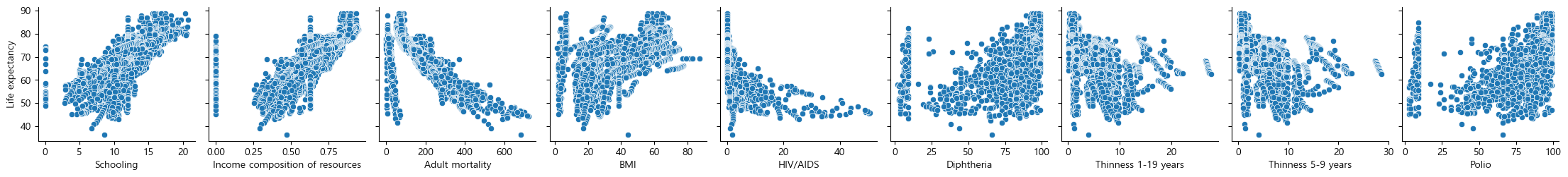
1.5. 모델 훈련 및 평가
이제 학습만 하면 된다.
X=life_df[col]
Y=life_df["Life expectancy"]
print(X.shape, type(X))
print(Y.shape, type(Y))
(2938, 9) <class 'pandas.core.frame.DataFrame'>
(2938,) <class 'pandas.core.series.Series'>훈련데이터와 테스트데이터를 나누자.
X_train, X_test, Y_train, Y_test=train_test_split(X, Y, random_state=42)이제 훈련시켜보자.
lr=LinearRegression()
lr.fit(X_train, Y_train)
훈련을 마쳤으니 평가의 차례다.
print("학습: ", lr.score(X_train, Y_train))
print("일반화: ", lr.score(X_test, Y_test))
학습: 0.8002007648036908
일반화: 0.7962053773778233전체적으로 낮긴하지만 잘 됐다.
1.6. 평가지표
이제 각 평가지표를 다 확인해보자.
Y_train_pred=lr.predict(X_train)
Y_test_pred=lr.predict(X_test)
이렇게 X_train의 예측값들과 X_test의 예측값들을 다 넣어준다.
그리고 이번에는 함수를 만들어서 사용하기 편하게 바꿔보자.
def regg_eval(model):
    Y_train_pred=lr.predict(X_train)
    Y_test_pred=lr.predict(X_test)

    print("학습 R2:", r2_score(Y_train, Y_train_pred))
    print("일반화 R2:", r2_score(Y_test, Y_test_pred), "\n")

    print("학습 MSE:", mean_squared_error(Y_train, Y_train_pred))
    print("일반화 MSE:", mean_squared_error(Y_test, Y_test_pred), "\n")

    print("학습 RMSE:", root_mean_squared_error(Y_train, Y_train_pred))
    print("일반화 RMSE:", root_mean_squared_error(Y_test, Y_test_pred), "\n")

    print("학습 MAE:", mean_absolute_error(Y_train, Y_train_pred))
    print("일반화 MAE:", mean_absolute_error(Y_test, Y_test_pred))
이렇게 만들고 앞서 만든 lr=LinearRegression() 을 이용하면,
regg_eval(lr)학습 R2: 0.8002007648036908
일반화 R2: 0.7962053773778233
학습 MSE: 18.065388279827335
일반화 MSE: 18.348077207731762
학습 RMSE: 4.250339784044017
일반화 RMSE: 4.283465560469906
학습 MAE: 3.1383510048400654
일반화 MAE: 3.107491734368549이렇게 결과가 잘 나왔는데,
이번에는 변수간에 스케일 차이가 있을 경우 처리하면 어떤 차이를 보이는지 확인해보자.
from sklearn.preprocessing import StandardScalerX_train, X_test, Y_train, Y_test=train_test_split(X, Y, random_state=42)
scaler=StandardScaler()
scaler.fit(X_train) # 표준편차, 평균
# Z-score
X_train_scaled=scaler.transform(X_train)
X_test_scaled=scaler.transform(X_test)
lr=LinearRegression()
lr.fit(X_train_scaled, Y_train)
print("학습: ", lr.score(X_train_scaled, Y_train))
print("일반화: ", lr.score(X_test_scaled, Y_test))
학습: 0.8002007648036908
일반화: 0.7962053773778238이렇게 별 차이는 없는데, 스케일을 사용하면 통일이 되니까 예측이 좀 빨라지니 스케일링해서 사용하는 게 좀 더 좋다.