Classification

• Qualitative variables take values in an unordered set $C$, such as
  $\text{eye color}\in\{\text{{brown, blue, green}}\}\\ \text{email}\in\{\text{spam, ham}\}$
• Given a feature vector $X$ and a qualitative response $Y$ taking values in the set $C$

  The Classification task is to build a function $C(X)$ that takes as input the feature vector $X$ and predicts its value for $Y$

• Often we are more interested in estimating the probabilities that $X$ belongs to each category in $C$.
  

Can we use Linear Regression?

• Suppose for the Default classification task that we code

  $Y = \begin{cases} 0 & \text{if \;\textcolor{red}{No}} \\ 1 & \text{if \;\textcolor{red}{Yes}} \end{cases}$

• Can we simply perform a linear regression of $Y$ on $X$ and classify as Yes if $\hat Y > 0.5$?

  • In this case of a binary outcome, linear regression does a good job as a classifier, and if equivalent to linear discriminant analysis which we discuss later
  • Since in the population $E(Y|X=x)=Pr(Y=1|X=x)$, we might think that regression is perfect for this task
  • However, linear regression might produce probabilities less than zero or bigger than one

    Logistic regression is more appropriate
    

• Now suppose that

  $Y = \begin{cases} 1 & \text{if \;\textcolor{red}{stroke}} \\ 2 & \text{if \;\textcolor{red}{drug overdose}} \\ 3 & \text{if \;\textcolor{red}{epileptic seizure}} \end{cases}$

• Linear regression is not appropriate here

  Multiclass Logistic Regression or Discriminant Analysis are more appropriate

Logistic Regression

• Let's write $p(X) = Pr(Y=1|X)$ for short and consider using $balance$ to predict $default$. Logistic regression uses the form
  $p(X) = \frac{e^{B_0+B_1X}}{1+e^{B_0+B_1X}}$
• $e\approx2.71828$ is a mathematical constant [Euler's number]
• $p(X)$ will have values between 0 and 1
• A bit of rearrangement gives : log odds or logit
  $\ln\left(\frac{p(X)}{1-p(X)}\right)=\beta_0+\beta_1X$

Maximum Likelihood

• This likelihood gives the probability of the observed zeros and ones in the data
• We pick $\beta_0$ and $\beta_1$ to maximize the likelihood of the observed data

Making Predictions

• What is estimated probability of $default$ for someone with a $balance$ of $1000?
  $\hat p(X) = \frac{e^{\hat\beta_0+\hat\beta_1X}}{1 +e^{\hat\beta_0+\hat\beta_1X}} = \frac{e^{-10.6513+0.0055\times100}}{1 + e^{-10.6513+0.0055\times100}} = 0.006$

Logistic Regression with several variables

Logistic Regression with more than two classes

• Multiclass logistic regression is also referred to as multinomial regression

Discriminant Analysis

• Here the approach is to model the distribution of $X$ in each of the classes separately, and then use Bayes theorem to flip things around and obtain $\text{Pr}(Y|X)$
• When we use Normal or Gaussian distributions for each class, this leads to linear or quadratic discriminant analysis

Bayes theorem for classification

• Bayes theorem

  $\text{Pr}(Y=k|X=x)=\frac{\text{Pr}(X=x|Y=k)\cdot\text{Pr}(Y=k)}{\text{Pr}(X=x)}$

• One writes this slightly differently for discriminant analysis:

  $\text{Pr}(Y=k|X=x)=\frac{\pi_kf_k(x)}{\sum_{l=1}^K\pi_lf_l(x)},\;\text{where}$
  • $f_k(x) = \text{Pr}(X=x|Y=k)$ is the density for $X$ in class $k$
  • $\pi_k=\text{Pr}(Y=k)$ is the marginal or prior probability for class $k$
    

• When the priors are different, we take them into account as well, and compare $\pi_kf_k(x)$.

• On the right, we favor the blue class - the decision boundary has shifted to the left

Why discriminant analysis?

• When the classes are well-separated, the parameter estimates for the logistic regression model are surprisingly unstable. But, Linear discriminant analysis does not suffer from this problem
• If $n$ is small and the distribution of the predictors $X$ is approximately normal in each of the classes, the linear discriminant model is again more stable than the logistic regression model
• Linear discriminant analysis is popular when we have more than two response classes, because it also provides low-dimensional views of the data

Linear Discriminant Analysis when p = 1(Uncorrelated)

• The Gaussian density has the form
  $f_k(x) = \frac{1}{\sqrt{2\pi}\sigma_k}e^{-\frac{1}{2}\left(\frac{x-\mu_k}{\sigma_k}\right)^2}$
• Here $\mu_k$ is the mean, and $\sigma_k^2$ the variance (in class $k$)
• We will assume that all the $\sigma_k=\sigma$ are the same
• Plugging this into Bayes formula, we got a rather complex expression for $p_k(x) = \text{Pr}(Y=k|X=x)$
  $p_k(x) = \frac{\pi_k \frac{1}{\sqrt{2\pi}\sigma} e^{-\frac{1}{2}\left(\frac{x - \mu_k}{\sigma}\right)^2}}{\sum_{l=1}^{K} \pi_l \frac{1}{\sqrt{2\pi}\sigma} e^{-\frac{1}{2}\left(\frac{x - \mu_l}{\sigma}\right)^2}}$

Discriminant functions

• To classify at the value $X=x$, we need to see which of the $p_k(x)$ is largest
• Taking logs, and discarding terms that do not depend on $k$, we see that this is equivalent to assigning $x$ to the class with the largest discriminant score:
  $\delta_k(x) = x \cdot \frac{\mu_k}{\sigma^2} - \frac{\mu_k^2}{2\sigma^2} + \log(\pi_k)$
• Note that $\delta_k(x)$ is a linear function of $x$
• If there are $K=2$ classes and $\pi_1=\pi_2=0.5$, then one can see that the decision boundary is at
  $x=\frac{\mu_1+\mu_2}{2} \hat{\pi}_k = \frac{n_k}{n} \\ \hat{\mu}_k = \frac{1}{n_k} \sum_{i: y_i = k} x_i \\ \hat{\sigma}^2 = \frac{1}{n - K} \sum_{k=1}^{K} \sum_{i: y_i = k} (x_i - \hat{\mu}_k)^2 \\ = \sum_{k=1}^{K} \frac{n_k - 1}{n - K} \cdot \hat{\sigma}_k^2$
• where $\hat{\sigma}_k^2 = \frac{1}{n_k - 1} \sum_{i: y_i = k} (x_i - \hat{\mu}_k)^2$ is the usual formula for the estimated variance in the $k$th class

Linear Discriminant Anaysis when p > 1(Correlated)

• $\text{Density: } f(x) = \frac{1}{(2\pi)^{p/2} |\Sigma|^{1/2}} e^{-\frac{1}{2} (x - \mu)^T \Sigma^{-1} (x - \mu)}$
• $\text{Discriminant function: } \delta_k(x) = \textcolor{red}{x^T \Sigma^{-1} \mu_k} - \frac{1}{2} \mu_k^T \Sigma^{-1} \mu_k + \log \pi_k$
  (Red : linear in $X$, other : constant)
• Despite its complex form:
  $\delta_k(x) = c_{k0} + c_{k1}x_1 + c_{k2}x_2 + \cdots + c_{kp}x_p \text{ — a linear function.}$

Fisher's Discriminant Plot

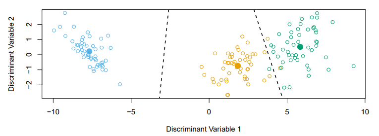
• When there are $K$ classes, linear discriminant analysis can be viewed exactly in a $K-1$ dimensional plot

  Because it essentially classifies to the closest centroid and they span a K-1 dimensional plane

• Even when $K > 3$, we can find the best 2-dimensional plance for visualizing the discriminant rule

From delta function to probabilities

• One we have estimates $\hat\delta_k(x)$, we can turn these into estimates for class probabilities:
  $\hat{\text{Pr}}(Y=k| X=x)=\frac{e^{\hat\delta_k(x)}}{\sum_{l=1}^Ke^{\hat\delta_l}(x)}$
• So classifying to the largest $\hat\delta_k(x)$ amounts to classifying to the class for which $\hat\text{Pr}(Y=k|X=x)$ is largest
• When $K=2$, we classify to class $2$ if $\hat\text{Pr}(Y=2|X=x) \geq 0.5$, else to class 1

Confusion Matrix

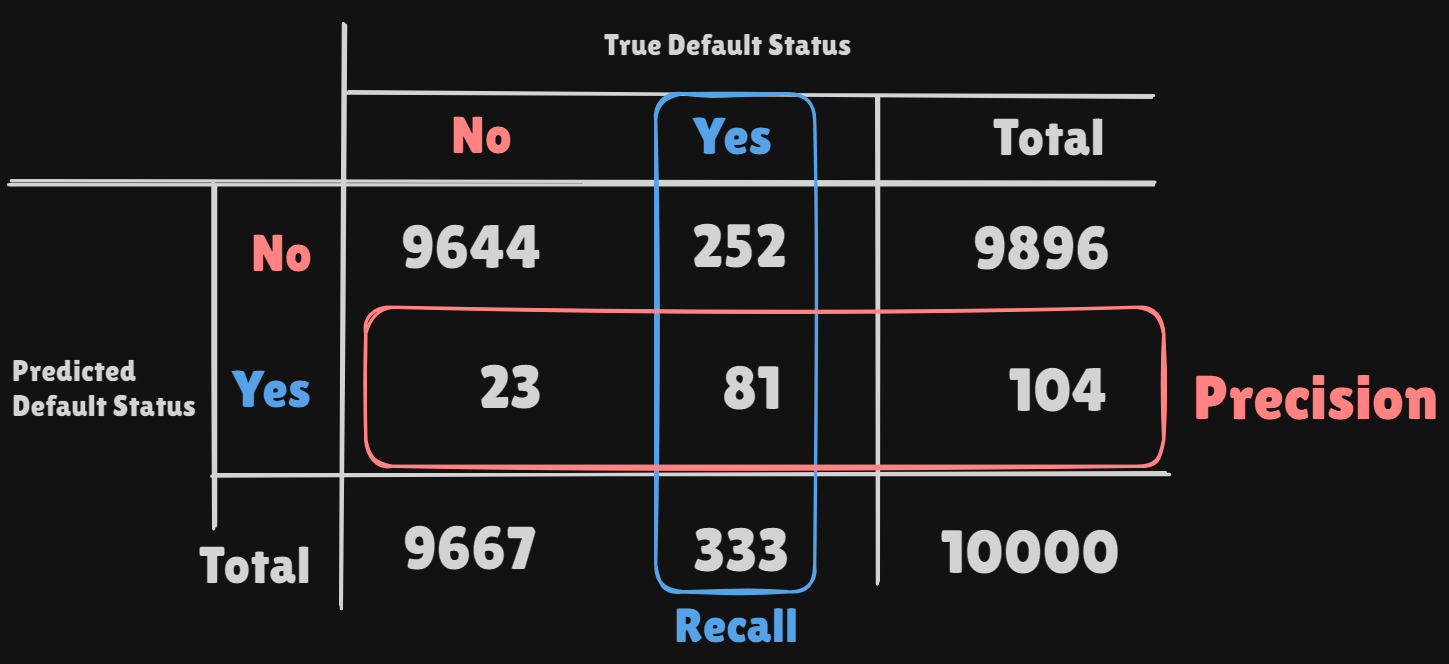
• misclassification rate : $(23 + 252) / 10000 = 2.75\%$
• precision : $81/104$
• recall : $252/333$
• False positive rate : The fraction of negative examples that are classified as positive - $0.2\%$ in example
• False negative rate : The fraction of positive examples that are classified as negative - $75.7\%$ in example
• We produced this table by classifying to class $Yes$ if
  $\hat\text{Pr}(Default=Yes|Balance,Student)\geq0.5$
  

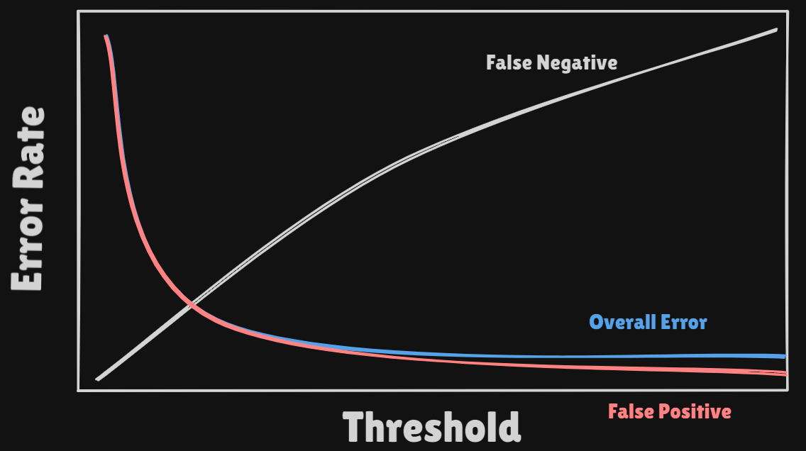
  • Lower Threshold : Higher False Positive and Lower False Negative
  • Higher Threshold : Lower False Positive and Higher False Negative
    
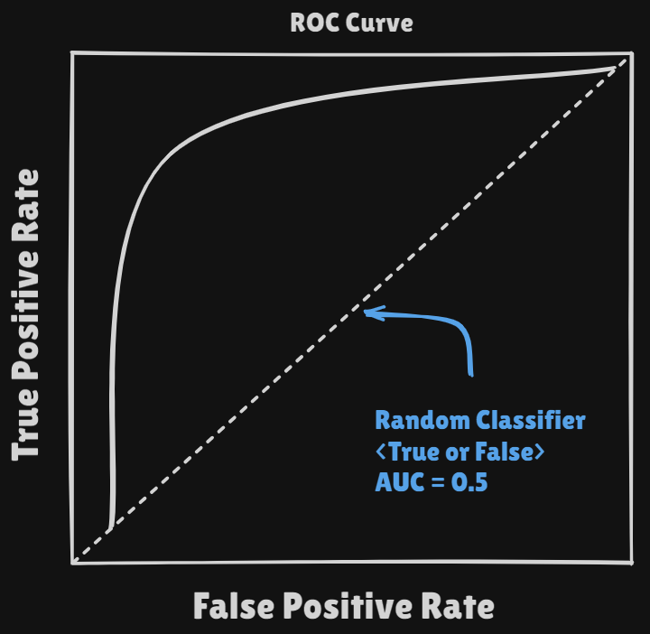
    With controlling the threshold we can get ROC Curve
  • If the classifier has good performance the AUC value goes near 1

Other forms of Discriminant Analysis

• With Gaussians but different $\sum_k$ in each class, we get quadratic discriminant analysis
• With Gaussians and same $\sum_k$ in each class, we get linear discriminant analysis
• With $f_k(x)=\prod_{j=1}^pf_{jk}(x_j)$ (conditional independence model) in each class we get naive Bayes. For Gaussian this means the $\sum_k$ are diagonal
  • $\sum_k$ : Covariance Matrix
    $\delta_k(x) = -\frac{1}{2}(x - \mu_k)^T \Sigma_k^{-1} (x - \mu_k) + \log \pi_k - \frac{1}{2} \log |\Sigma_k|$

Naive Bayes

• Assume features are independent in each class
• Useful when $p$ is large, and so multivariate methods like QDA and even LDA break down
• Gaussian naive Bayes assumes each $\sum_k$ is diagonal:
  $\delta_k(x) \propto \log \left[ \pi_k \prod_{j=1}^{p} f_{kj}(x_j) \right] \\= -\frac{1}{2} \sum_{j=1}^{p} \left[ \frac{(x_j - \mu_{kj})^2}{\sigma_{kj}^2} + \log \sigma_{kj}^2 \right] + \log \pi_k$
• For mixed feature vectors(qualitative and quantitative)

  If $X_j$ is qualitative, replace $f_{kj}(x_j)$ with probability mass function (histogram) over discrete categories

Logistic Regression versus LDA

• For a two-class problem, one can show that for LDA
  $\log \left( \frac{p_1(x)}{1 - p_1(x)} \right) = \log \left( \frac{p_1(x)}{p_2(x)} \right) = c_0 + c_1 x_1 + \cdots + c_p x_p$
• So it has same form as logistic regression
• The difference is in how the parameters are estimated
  • Logistic Regression uses the conditional likelihood based on $\text{Pr}(Y|X)$ (discriminative learning)
  • LDA uses the full likelihood based on $\text{Pr}(X,Y)$ (generative learning)
• Logistic Regression can also fit quadratic boundaries like QDA, by explicitly including quadratic terms in the model

Multinomial Logistic Regression

• The simplest representation uses different linear functions for each class, combined with the softmax function to form probabilities
  $\Pr(Y = k \mid X = x) = \frac{e^{\beta_{k0} + \beta_{k1}x_1 + \cdots + \beta_{kp}x_p}}{\sum_{l=1}^{K} e^{\beta_{l0} + \beta_{l1}x_1 + \cdots + \beta_{lp}x_p}}.$
• There is a rebundancy here; we really only need $K-1$ functions
• We fit by maximizing the multinomial log likelihood (cross-entropy) - a generalization of the binomial

Generative Models and Naive Bayes

• Logistic regression models $\text{Pr}(Y=k|X=x)$ directly, via the logistic function

• Similarly the multinomial logistic regression uses the softmax function

• These all model the conditional distribution of $Y$ given $X$

• By contrast generative models start with the conditional distribution of $X$ given $Y$, and then use Bayes formula to turn things around:

  $\Pr(Y = k \mid X = x) = \frac{\pi_k f_k(x)}{\sum_{l=1}^{K} \pi_l f_l(x)}.$

• $f_k(x)$ is the density of $X$ given $Y=k$

• $\pi_k=\text{Pr}(Y=k)$ is the marginal probability that $Y$ is in class $k$

• Linear and Quadratic discriminant analysis derive from generative models, where $f_k(x)$ are Gaussian

• Often useful if some classes are well seperated - a situation where logistic regression is unstable

• Naive Bayes assumes that the densities $f_k(x)$ in each class

  Factor

  $f_k(x) = f_{k1}(x_1) \times f_{k2}(x_2) \times \cdots \times f_{kp}(x_p)$

• Equivalently this assumes that the features are independent within each class

• Then using Bayes formula:

  $\Pr(Y = k \mid X = x) = \frac{\pi_k \times f_{k1}(x_1) \times f_{k2}(x_2) \times \cdots \times f_{kp}(x_p)}{\sum_{l=1}^{K} \pi_l \times f_{l1}(x_1) \times f_{l2}(x_2) \times \cdots \times f_{lp}(x_p)}$

• $f_{k1}(x_1) \times f_{k2}(x_2) \times \cdots \times f_{kp}(x_p)$ : Probability that the value could be found by each distribution

Why independence assumption for naive bayes?

• Difficult to specify and model high-dimensional densities. Much easier to specify one-dimensional densities
• Can handle mixed features
  • If feature $j$ is quantitative, can model as univariate Gaussian. We estimate $\mu_{jk}$ and $\sigma_{jk}^2$ from the data, and then plug into Gaussian density formula for $f_{jk}(x_j)$
  • Alternatively, can use a histogram estimate of the density, and directly estimate $f_{jk}(x_j)$ by the proportion of observations in the bin into which $x_j$ falls
  • If feature $j$ is qualitative, can simply model the proportion in each category
    
    $\text{Pr}(Y=1|X=x^*)=0.944 \text{ and Pr}(Y=2|X=x^*)=0.056$

Naive Bayes and GAMs

• Hence, the Naive Bayes model takes the form of a generalized additive model from later Chapter

Generalized Linear Models

• Generalized linear models provide a unified framework for dealing with many different response types(non-negative responses, skewed distributions, and more)
  
• In left plot we see that the variance mostly increases with the mean
• Taking log($bikers$) alleviates this, but has its own problems: e.g. predictions are on the wrong scale, and some counts are zero

Poisson Regression Model

• Poisson Distribution is useful for modeling counts:
  $\text{Pr}(Y=k)=\frac{e^{-\lambda}\lambda^k}{k!} \text{ for k = }0,1,2\dots$
• $\lambda=E(Y)=\text{Var}(Y)$ - there is a mean/variance dependence
• With covariates, we model
  $\log(\lambda(X_1, \ldots, X_p)) = \beta_0 + \beta_1 X_1 + \cdots + \beta_p X_p$
  or equivalently
  $\text{or equivalently} \quad \lambda(X_1, \ldots, X_p) = e^{\beta_0 + \beta_1 X_1 + \cdots + \beta_p X_p}.$
• Model automatically gurantees that the predictions are non-negative

Three GLMs

• We have covered three GLMs : Gaussian, Binomial and Poisson
• They each have a characteristic link function. This it the transformation of the mean that is represented by a linear model
  $\eta(\mathbb{E}(Y \mid X_1, X_2, \ldots, X_p)) = \beta_0 + \beta_1 X_1 + \cdots + \beta_p X_p$
  • linear : $\eta(\mu)=\mu$
  • logistic : $\eta(\mu=\log(\mu(1-\mu))$
  • Poisson regression : $\eta(\mu)=\log(\mu)$
• They also each have characteristic variance functions
• The modls are fit by maximum-likelihood

All Contents written based on GIST - Machine Learning & Deep Learning Lesson(Instructor : Prof. sun-dong. Kim)