Linear regression

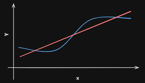
• Linear regression is a simple approach to supervised learning. It assumes that the dependence of
  $Y$ on $X_1, X_2, \cdots , X_p$ is linear.

  True regression functions are never linear!
  

• Although it may seem overly simplistic, linear regression is extremely useful both conceptually and practically.

Simple linear regression using a single predictor X

• We assume a model
  $Y=B_0+B_1X+\epsilon,\;E[\epsilon]=0$

  where $\beta_0$ and $\beta_1$ are two unkown constants that represent the intercept and slope, also known as coefficients or parameters, and $\epsilon$ is the error term

• Where $\hat y$ indicates a prediction of $Y$ on the basis of $X=x$.

  The $\textcolor{red}{hat}$ symbol denotes an estimated value

Estimation of the parameters by least squares

• Let $\hat{y_i} =\hat\beta_0+\hat \beta_1x_i$ be the prediction for $Y$ based on the $i$th value of $X$.

  Then $e_i =y_i-\hat y_i$ represents the $i$th residual

• We define the residual sum of squares(RSS) as

  $RSS = e^2_1+e^2_2+\cdots+e^2_n$
  or
  $RSS = (y_1-\hat \beta_0 -\hat \beta_1x_1)^2 + (y_2-\hat \beta_0-\hat \beta_1x_2)^2+\cdots+(y_n-\hat \beta_0-\hat \beta_1x_n)^2$

• The least squares approach chooses $\hat \beta_0$ and $\hat \beta_1$ to minimize the $RSS$.

  The minimizing values can be shown to be

  $\hat \beta_1 = \dfrac{\displaystyle \sum_{i=1}^{n} (x_i-\bar x)(y_i -\bar y)}{\displaystyle \sum_{i=1}^{n}(x_i-\bar x)^2}\\[0.5cm] \hat \beta_0 =\bar y-\hat \beta_1\bar x$

  where the $\bar y =\frac{1}{n}\displaystyle\sum_{i=1}^{n}y_i,\quad\bar x=\frac{1}{n}\displaystyle\sum_{i=1}^{n}x_i$ are the sample means

Assessing the Accuracy of the Coefficient Estimates

• The standard error of an estimator reflects how it varies under repeated sampling.

  $SE(\hat\beta_1)^2=\dfrac{\sigma^2}{\displaystyle\sum_{i=1}^n(x_i-\bar x)^2},\quad SE(\bar \beta_0)^2=\sigma^2\left[\dfrac{1}{n} + \dfrac{\bar x^2}{\displaystyle\sum_{i=1}^n(x_i-\bar x)^2}\right] \\where, \sigma^2=Var(\epsilon)$

• These standard errors can be used to compute confidence intervals

• A 95% confidence interval is defined as a range of values such that with 95% probability, the range will contain the true unknown value of the parameter. It has the form

  $\hat \beta_1 \pm2\times SE(\hat \beta_1)$

  There is approximately a 95% chance that the interval

  $[\hat \beta_1-2\times SE(\hat \beta_1),\;\hat \beta_1+2\times SE(\hat \beta_1)]$

  It will contain the true value of $\beta_1$

• For example, for the advertising data, the 95% confidence interval for $\beta_1$ is $[0.042, 0.053]$

Hypothesis testing

• The most common hypothesis testing involves testing the null hypothesis of

  $H_0$	There is no relationship between $X$ and $Y$ versus the alternative hypothesis
  $H_1$	There is some relationship between $X$ and $Y$

• Mathematically, this corresponds to testing
  $H_0:\beta_1=0$ versus $H_A:\beta_1\neq0$

• Since if $\beta_1=0$ then the model reduces to $Y=\beta_0+\epsilon$, and $X$ is not associated with $Y$

• To test the null hypothesis, we compute a t-statistic, given by

  $t=\dfrac{\hat \beta_1-0}{SE(\hat\beta_1)}$

• This will have a t-distribution with n-2 degrees of freedom, assuming $\beta_1=0$.

• p-value : probability of observing any value equal to $|t|$ or larger

  	Coefficient	Std. Error	t-statistic	p-value
  $Intercept$	7.0325	0.4578	15.36	<0.0001
  $TV$	0.0475	0.0027	17.67	<0.0001

Assessing the Overall Accuracy of the Model

• We compute the Residual Standard Error

  $RSE=\sqrt{\dfrac{1}{n-2}\;RSS}=\sqrt{\dfrac{1}{n-2}\displaystyle\sum_{i=1}^n(y_i-\hat y_i)^2}$

  where the residual sum-of-squares is RSS $=\displaystyle\sum_{i=1}^n(y_i-\hat y_i)^2$

• $R-squared$ or fraction of variance explained is

  $R^2=\dfrac{TSS-RSS}{TSS}=1-\dfrac{RSS}{TSS}$

  where the total sum of squares(TSS) $=\displaystyle\sum_{i=1}^n(y_i-\bar y)^2$

• It can be shown that in this simple linear regression setting that $R^2=r^2$, where $r$ is the correlation between 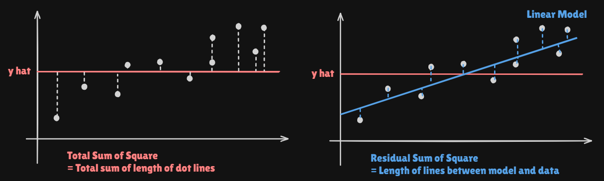$X$ and $Y$:

  $r=\dfrac{Cov_{xy}}{Cov_{xx}\;Cov_{yy}}=\dfrac{\displaystyle\sum_{i=1}^n(x_i-\bar x)(y_i-\bar y)}{\sqrt{\displaystyle\sum_{i=1}^n(x_i-\bar x)^2}\sqrt{\displaystyle\sum_{i=1}^n(y_i-\bar y)^2}}$

  

Multi Linear Regression

• Here our model is

  $Y=\beta_0+\beta_1X_1+\beta_2X_2+\cdots+\beta_pX_p+\epsilon$

• We interpret $\beta_j$ as the average effect on $Y$ of a one unit increase in $X_j$, holding all other predictors fixed

Interpreting regression coefficients

• The ideal scenario is when the predictors are uncorrelated : a balanced design
  • Each coefficient can be estimated and tested separately
• Correlations amongst predictors cause problems :
  • The variance of all coefficients tends to increase, sometimes dramatically
  • Interpretations become hazardous - when $X_j$ changes, everything else changes
• Claims of causality should be avoided for observational data

Estimation and Prediction for Multiple Regression

• Given estimates $\hat \beta_0,\hat \beta_1,\cdots,\hat \beta_p$ we can make predictions using the formula

  $\hat y =\hat \beta_0+\hat \beta_1x_1+\hat \beta_2x_2+\cdots+\hat \beta_px_p$

• We estimate $\beta_0,\beta_1,\cdots,\beta_p$ as the values that minimize the sum of squared residuals

  $RSS =\displaystyle\sum_{i=1}^n(y_i-\hat y_i)^2\\[0.5cm] =\displaystyle\sum_{i=1}^n(y_i-\hat \beta_0-\hat \beta_1x_{i1}-\hat \beta_2x_{i2}-\cdots-\hat \beta_px_{ip})^2$

Some important questions

1. Is at least one of the predictors $X_1,X_2,\cdots,X_p$ useful in predicting the response
2. Do all the predictors help to explain $Y$, or is only a subset of the predictors useful?
3. How well does the model fit the data?
4. Given a set of predictor values, what response value should we predict, and how accurate is our prediction?

Is at least one predictor useful?

• For the first question, we can use the F-statistic

  $F=\dfrac{(TSS-RSS)/p}{RSS/(n-p-1)}\sim F_{p,\;n-p-1}$

• It decits how effective each predictor was or at least one effective
  • At least on coefficient Effective? $\rightarrow$ $\textcolor{red}{High}\;F-statistics$
  • No Predictor Effective? $\rightarrow$ $\textcolor{blue}{Low}\;F-statistics$

Deciding on the important variable

• The most direct approach is called all subsets or best subsets regression
  • We compute the least squares fit for all possible subsets and then choose between them based on some criterion that balances training error with model size
• But, we can not invest resources for $2^p$ of them. We should find optimized subsets

Forward Selection

• Begin with the null model
• Fit $p$ simple linear regression and add to the null model the variable that result in the lowest RSS
• Continue until some stopping rule is satisfied

Backward Selection

• Start with all variables in the model
• Remove the variables with the largest p-value
• The new $(p-1)$ variable model is fit, and the variable with the largest p-value is removed
• Continue until some stopping rule is reached

Other Considerations in the Regression Model

Qualitative Predictors

• Some predictors are not quantitative but the qualitative, taking a discrete set of values
• These are also called categorical predictors or factor variables
• We can express these qualitative predictors like this

  $x_i = \begin{cases} 1 & \text{if ith person is female} \\ 0 & \text{if ith person is male} \end{cases}\\[0.5cm] y_i=\beta_0+\beta_1x_i+\epsilon_i=\begin{cases} \beta_0+\beta_1+\epsilon_i & \text{if ith person is female}\\ \beta_0+\epsilon_i & \text{if ith person is male} \end{cases}$

Qualitative predictors with more than two levels

• With more than two levels, we create additional dummy variables

  $x_i1 = \begin{cases} 1 & \text{if ith person is Asian} \\ 0 & \text{if ith person is not Asian} \end{cases}\\[0.3cm] x_i2 = \begin{cases} 1 & \text{if ith person is Caucasian} \\ 0 & \text{if ith person is not Caucasian} \end{cases}\\[0.5cm] y_i=\beta_0+\beta_1x_{i1}+ \beta_2x_{i2}+\epsilon_i=\begin{cases} \beta_0+\beta_1+\epsilon_i & \text{if ith person is Asian}\\ \beta_0+\beta_2+\epsilon_i & \text{if ith person is Caucasian}\\ \beta_0+\epsilon_i & \text{if ith person is AA} \end{cases}$

• There will always be one fewer dummy variable than the number of levels

• Baseline : What do you want to set as intercept is very important

Extensions of the Linear Model

• Removing the additive assumption : interactions and nonlinearity

Interactions

• In out previous analysis of the Advertising data, we assumed that the effect on sales of increasing one advertising medium is independent of the amount spent on the other media
• But suppose that spending money on rdio advertising actually increases the effectiveness of TV advertising
• In marketting, this is known as a synergy effect, and in statistics it is referred to as an interaction effect
• Then we can deal with this problem by transforming the formula

  $\text{sales}=\beta_0+\beta_1\times\text{TV} +\beta_2\times\text{radio}+\beta_3\times(\text{radio}\times\text{TV})+\epsilon\\ =\beta_0+(\beta_1+\beta_3\times\text{radio})\times\text{TV}+\beta_2\times\text{radio}+\epsilon$

Hierarchy

• Sometimes it is the case that an interaction term has a very small p-value, but the associated main effects do not
• The hierarchy principle :

  • If we include an interaction in a model, we should also include the main effects, even if the p-values associated with their coefficients are not significant

• The rationale for this principle is that interactions are hard to interpret in a model without main effects
• Specifically, the interaction terms also contain main effects, if the model has no main effect terms

Interactions between qualitative and quantitative variables

• Without an interaction term, the model takes the form

  $\text{balance}_i \approx \beta_0 + \beta_1 \times \text{income}_i + \begin{cases} \beta_2 & \text{if $i$th person is a student} \\ 0 & \text{if $i$th person is not a student} \end{cases} \\ = \beta_1 \times \text{income}_i + \begin{cases} \beta_0 + \beta_2 & \text{if $i$th person is a student} \\ \beta_0 & \text{if $i$th person is not a student} \end{cases}$

• With interactions, it takes the form

  $\text{balance}_i \approx \beta_0 + \beta_1 \times \text{income}_i + \begin{cases} \beta_2 + \beta_3 \times \text{income}_i & \text{if student} \\ 0 & \text{if not student} \end{cases} \\ = \begin{cases} (\beta_0 + \beta_2) + (\beta_1 + \beta_3) \times \text{income}_i & \text{if student} \\ \beta_0 + \beta_1 \times \text{income}_i & \text{if not student} \end{cases}$

  

  • Same Slope $\rightarrow$ No interaction
  • Different Slope $\rightarrow$ With an interaction

Non-Linear effects of predictors

• Some Non-Linear structure might be more effective

  $\text{mpg} =\beta_0+\beta_1\times\text{horsepower}+\beta_2\times\text{horsepower}^2+\epsilon$

What we did not cover

• Outliers
• Non-constant variance of error terms
• High leverage points
• Collinearity

Next : Generalization of the Linear Model

• Classification problems : logistic regression, support vector machines
• Non-linearity : kernal smoothing, splines and generalized additive models : nearest neighbor methods
• Interactions : Tree-based methods, bagging, random forests and boosting
  • These also capture non-linearities
• Regularized fitting : Ridge regression and Lasso

All Contents written based on GIST - Machine Learning & Deep Learning Lesson(Instructor : Prof. sun-dong. Kim)