PCA(Principal Component Analysis) is one of well-known dimensionality reduction techniques. Simply put, we are representing 100-dimensional data with three-dimensional data. Before we get to the complicated part, let's first find out why we should reduce dimensionality.

Why do we reduce dimensionality?

Curse of Dimensionality

Curse of dimensionality is one of the main reasons why we reduce dimensionality. As the catchy name suggests, it means the increase of dimensionality is not that preferable.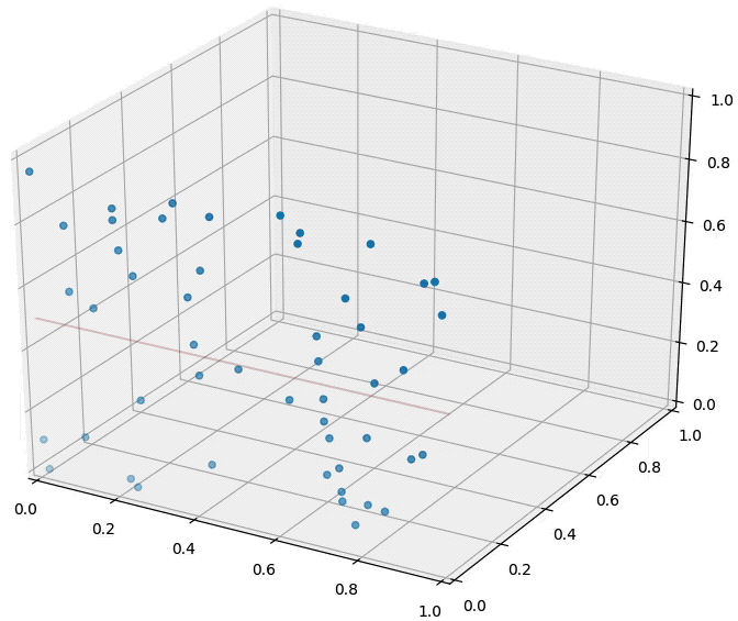Image source

As shown above, the data densely distributed in two-dimensional space are distributed relatively sparsely in three-dimensional space. In other words, as the dimensionality increases, the data needed for explanation increases rapidly. Therefore, if the dimensionality of data is higher than necessary, it becomes more difficult to train a model (too little data given for the dimensionality). This is why we use dimensionality-reduced inputs for a model when the dimensionality of input is too high.

Data Visualization

Dimensionality reduction is also used in data visualization. Suppose we just finished a clustering task on 100-dimensional data. In order to "see" if clustering is well performed, 100-dimensional data should be reduced to two-dimensional or three-dimensional data while maintaining the characteristics of data as much as possible. This is when dimensionality reduction techniques such as PCA are used.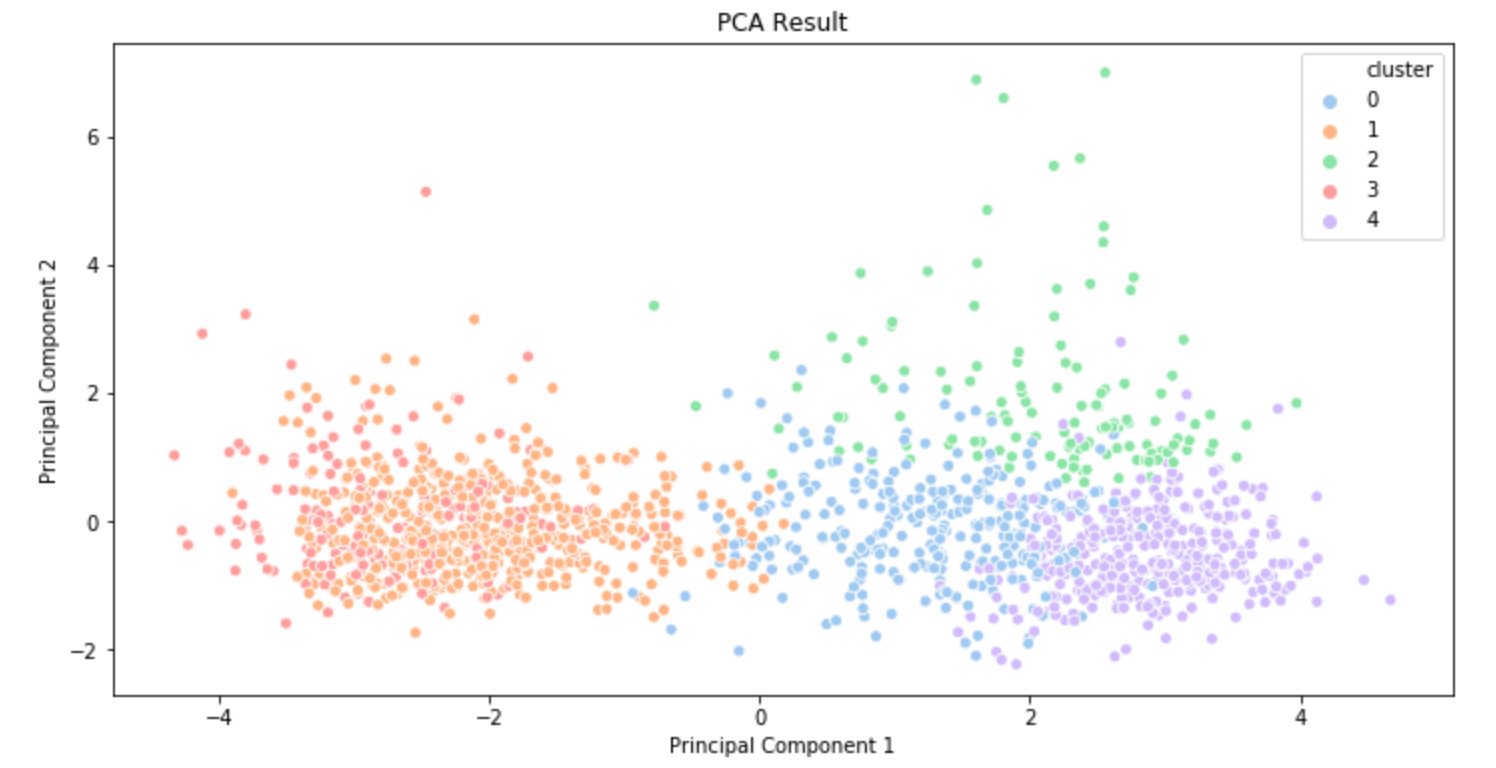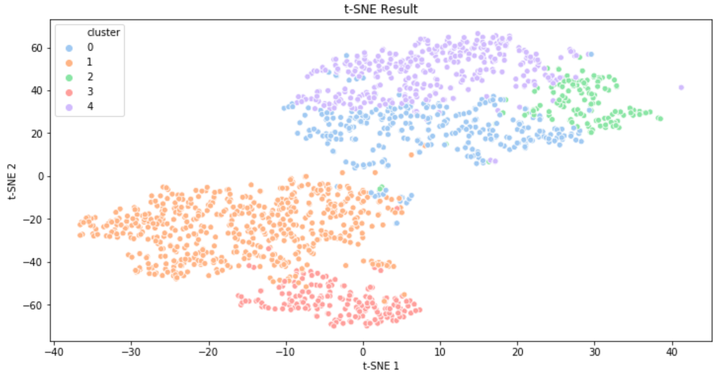The plots above are the clustering results of music data that I created a few months ago. The first result was visualized using PCA and the second result was created using t-SNE(t-distributed Stochastic Neighbor Embedding). (t-SNE is also a commonly used dimensionality reduction technique. You can get some information about t-SNE in this post.

How PCA Works

Basic Idea

The fundamental idea of PCA is maintaining the characteristics of data. Let's say that a set of two-dimensional data is given as follows.Suppose we reduce the data to one-dimensional data. What does it mean to reduce dimensionality while maintaining the characteristics of the data?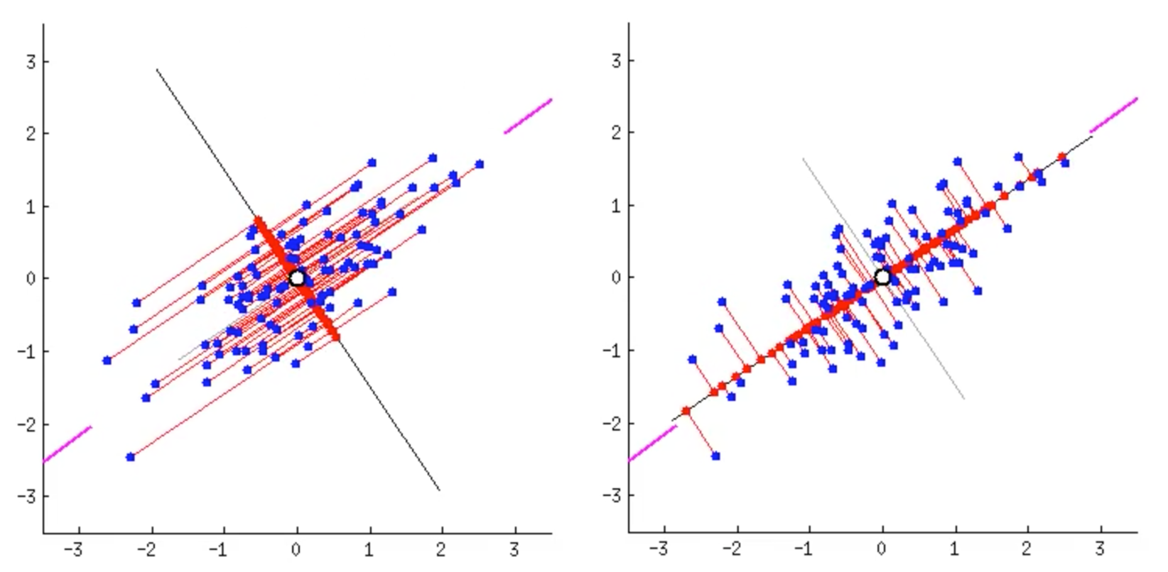Image source

The plots above show two different cases of dimensionality reduction(blue dots to red dots). Projection is used in both cases, yet the directions of the projection are different. In the left case, the projected data(red dots) are densely concentrated in the center. Even the distant data points are projected close to other points. But the situation on the right is different. The projected data are quite widely distributed on the black line (variance is large). In other words, the characteristics of data is well preserved in the right case.

Mathematical Interpretation

So, the key is maintaining the characteristics of data. As mentioned above, it can be done by keeping the variance of data to the maximum. Since the basic ideas have been organized, let's get into the math part.

Let's say we have $n$ $d$-dimensional data. If we say that the first vector to project the data (black line in the example above) is $u$, the problem can be summarized as follows.

To solve this problem, we first need to centralize $X$.

Centralizing simply means moving the whole data to the origin. Centralizing only moves the location of data and does not change the overall shape of the data. Since we only care about the direction of $u_1$, we may use $\tilde{X}$ instead of $X$. Therefore the optimization problem can be rewritten as below.

Let's look at $u^T\tilde{X}$ for a moment. $u^T\tilde{X}$ can be written ($\tilde{x_i}$ is the $i$-th column vector of $\tilde{X}$)

The expectation of $u^T\tilde{X}$ is thus

Since $\tilde{X}$ is a centralized matrix, the value of $\tilde{x_{1i}}+\dots+\tilde{x_{ni}}$ is zero. Therefore $E(u^T\tilde{X})$ equals zero. Now let's get back to the original problem.

Since $u^TSu$ is a quadratic form, we cannot find $u_1$ without any constraint. But as mentioned above, we only care about the direction of $u_1$. Thus, the length of $u_1$ can be set to 1. Using Lagrangian multiplier method,

Let's apply the result to the optimization problem.

Voilà! The $u_1$ we need is the vector that maximizes $\lambda$. Since $\lambda$ is an eigenvalue of $S$($=Var(\tilde{X})$) according to (1), $u_1$ is the eigenvector of the covariance matrix of $\tilde{X}$ corresponding to the largest eigenvalue. Such $u_1$ is called the first principal component. The second principal component is the vector that is orthogonal to the first principal component and maximizes the variance of the projected data (you can get the rest of the principal components in the same way).

How PCA is Related to SVD

PCA is also a concept deeply related to SVD(Singular Value Decomposition).

$U$ consists of the eigenvectors of $XX^T$ and $V$ consists of the eigenvectors of $X^TX$. What happens if we centralize $X$? (The $U$,$\Sigma$,$V$ below are different from the $U$,$\Sigma$,$V$ above, but for convenience they are denoted as $U$,$\Sigma$,$V$)

The column vectors of $U$ will be the eigenvectors of $\tilde{X}\tilde{X}^T$. Yes, the column vectors of $U$ are actually the eigenvectors of the covariance matrix of $\tilde{X}$. If the singular values in $\Sigma$ are listed in descending order, the first column vector of $U$ will be the first principal component of $X$. Simply put, we can get the principal components of $X$ by implementing SVD on centralized $X$.

---

So far, we have looked at the most basic form of PCA. There are some advanced PCA techniques that are suitable for particular cases - one example is dual PCA which is used when the value of $d$ is much greater than $n$ (when the dimensionality is much higher than the number of data). This lecture video will be quite helpful if you want to know additional PCA techniques.