[paper-review] Bottom-up Object Detection by Grouping Extreme and Center Points
Paper Review
Zhou, Xingyi, Jiacheng Zhuo, and Philipp Krahenbuhl. "Bottom-up object detection by grouping extreme and center points." Proceedings of the IEEE/CVF Conference on Computer Vision and Pattern Recognition. 2019.
3. Preliminaries
Extreme and center points
- 일반적으로 bounding box를 annotate할 때, 대부분 목표 물체 주변의 배경을 클릭하기 때문에 오류를 범하기 쉽다.
- 하지만, Extreme points는 목표 물체를 직접 클릭하기 때문에 오류를 범하는 일이 적다. 여기에 추가 계산을 통해 Center point를 지정한다.
CornerNet
- CornetNet은 HourglassNet을 통한 keypoint estimation을 사용해 object detection을 수행한 모델이다.
- 이 모델은 bounding box의 양 모서리를 두 쌍의 heatmap으로 예측했다.
- corner의 positive location이 negative location보다 극단적으로 수가 적기 때문에 corner를 예측하는 데 focal loss를 사용했다.
- : 한 이미지 안의 물체의 수
- : Focal Loss의 hyper-parameter, 논문에서는 각각 2, 4를 사용함.
- : 채널 에 대한 위치 의 예측 heatmap 값
- : 채널 에 대한 위치 의 ground truth heatmap 값
- HourglassNet이 down-sampling하며 잃어버리는 정보들을 조정해주는 offset의 개념을 추가하였다.
- offset map은 smooth L1 Loss를 통해 학습된다.
- : 여러 모서리 중 모서리 의 각각 좌표
- : down-sampling factor, 논문에서는 4
- extreme points를 찾는 데 CornerNet의 아키텍처와 loss를 사용했지만, CornerNet의 Associative embedding에 해당하는 loss는 사용하지 않고 후에 서술할 Center Grouping으로 대체했다.
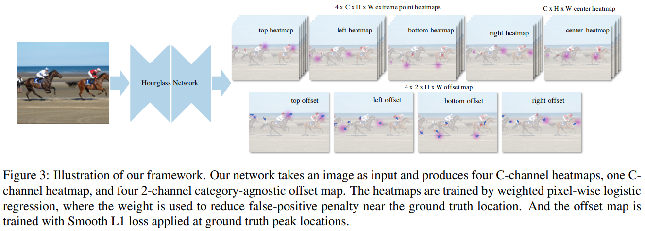
4. ExtremeNet for Object detection
- ExtremeNet은 CornerNet에서 HourglassNet을 기반으로 하는 것처럼 동일하게 사용하고 있다.
- HourglassNet의 결과물은 아래와 같다.
- 의 extreme points의 heatmap
- 는 클래스의 수
- 의 offset map
- 여기서 말하는 offset은 extreme points의 위치를 올바르게 조정해주는 요소들이다.
- 의 extreme points의 heatmap
4.1. Center Grouping
- HourglassNet의 결과물들이 각기 따로따로 있기 때문에 이들을 묶어주어야 한다.
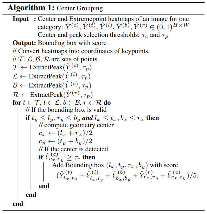
- Center Grouping 알고리즘의 입력 값은 아래와 같다.
- Center point heatmap
- 각각 top, left, bottom, right의 extreme point heatmap
- threshold로 사용될
- ExtractPeak : 각각 extreme point heatmap에서 주변 픽셀 값보다 보다 큰 픽셀 값을 peak라고 한다.
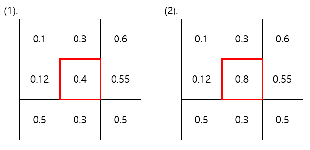
- (1) 그림은 주변 픽셀 값보다 충분히 큰 값()을 가지지 못하므로 peak가 아니다
- (2) 그림은 주변 픽셀 값보다 충분히 큰 값()을 가지므로 peak이다.
- 이렇게 모든 peak값 집합 에 대해서 Center point를 계산한다.
- 가 보다 크면 물체로 인식했다고 판단한다.
4.2. Ghost box suppression
- 같은 클래스를 갖는 세 물체가 나란히 있는 이미지의 경우에는 높은 확률로 "Ghost box"가 생긴다고 한다.
- Ghost box: 세 물체 중 가운데 물체의 extreme point들을 올바르게 잡지않고 인접한 다른 두 물체의 extreme points를 잡아 Grouping하여 세 물체를 한 번에 담는 bounding box를 말한다.
- 이 Ghost box들을 soft non-maxima suppression으로 제거했다.
4.3. Edge aggregation
- 대형버스 같은 직사각형 형태의 물체들의 extreme points는 그 물체의 가장자리를 따라 존재하는 다른 지점들도 extreme points로 간주할 수 있다.
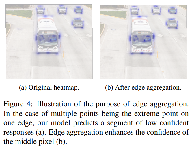
- 이와 같은 이유로 값이 큰 한 지점만 extreme point로 하지않고 값이 작은 여러 지점을 extreme point로 예측하도록 했다.
- 을 extreme point라고 할 때, 수직, 수평선을 따라 있는 픽셀 영역을 라고 표기하면
- 음수인 (왼쪽, 아랫방향), 양수인 (오른쪽, 윗방향)에 대하여 을 만족하는 값을 찾을 때까지 쭉 양옆으로 퍼지면서 아래의 가중치로 Edge aggregation을 적용한다.
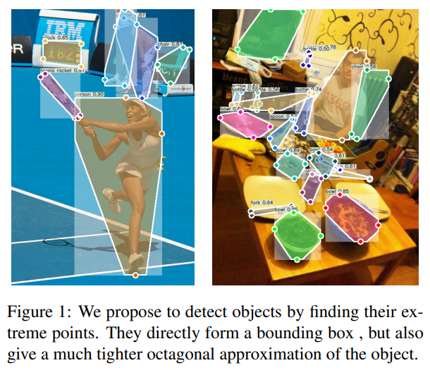
4.4. Extreme Instance Segmentation
-
extreme points로 bounding box를 나타내는 과정을 서술하고 있다.
We propose a simple method to approximate the object mask using extreme points by creating an octagon whose edges are centered on the extreme points. Specifically, for an extreme point, we extend it in both directions on its corresponding edge to a segment of 1/4 of the entire edge length. The segment is truncated when it meets a corner. We then connect the end points of the four segments to form the octagon. See Figure 1 for an example.
-
Edge aggregation을 거친 edge의 총 길이의 1/4을 box 길이로 한다는 의미인 것 같다.
-
추가적으로 instance segmentation에 사용되는 DEXTR 사전 학습 모델의 입력 값으로 extreme points를 주었을 때, segmentation 실험 결과도 관찰했다.
5. Experiments
- MS COCO dataset
train2017(118K images, 860K annotated objects)을 학습에 사용val2017(5K images, 36K annotated objects)을 ablation 연구에 사용test-dev(20K images)를 이전 연구들과의 비교 연구에 사용
- 평가척도
- : IOU threshold 0.5일 때 average precision
- : IOU threshold 0.75일 때 average precision
- : IOU threshold 0.5~1일 때 average precision
- : 물체의 크기에 따른 값
5.1. Extreme point annotations
- COCO에는 extreme point annotation이 없기 때문에 만들었다.
- COCO의 segmentation annotations 영역에서 한 edge가 평행하거나 3도 미만일 경우 그 edge의 중심점을 extreme point로 지정했다.
5.4. Ablation studies
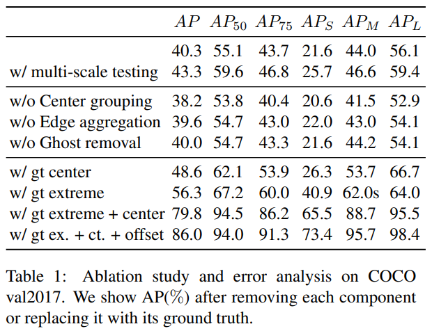
- 논문의 주요 요소인 Center grouping, Edge aggregation, Ghost removal을 제외하면서 결과를 비교.
- 각 요소의 영향력을 파악하기 위해 gt(ground truth)값을 주면서 결과를 비교
with gt center모델의 상승폭이 타 모델에 비해 적은 것을 보았을 때, center heatmap의 학습이 잘 이루어진다고 볼 수 있다.with gt extreme모델의 결과를 볼 때 extreme point heatmap을 알려주면 16.3% 상승을 볼 수 있다.with gt extreme+center의 결과를 통해, 5개의 모든 heatmap을 모델에 알려주면 엄청난 성능 향상이 있었고, 이는 extreme, center heatmap 모두 개선할 점이 있다고 볼 수 있다.
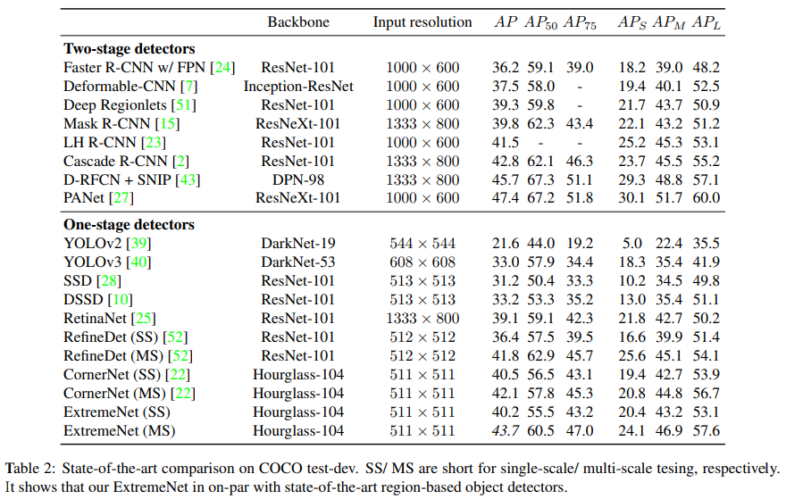
5.5. State-of-the-art comparisons
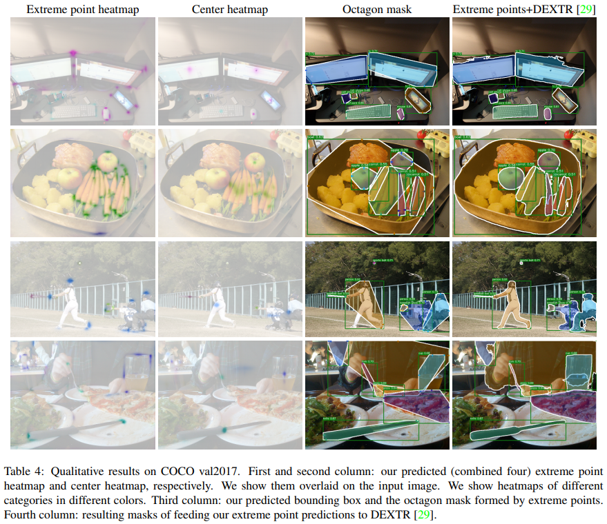
Qualitative results