Paper : Multi-Modal Unsupervised Image-to-Image Translation (Xun Huang, Ming-Yu Liu, Serge Belongie, Jan Kautz / ECCV 2018)

• Motivation : Cycle-GAN을 이용해서 Image-to-Image translation을 시도하고 있었는데, 이 방법은 target distribution을 one-to-one mapping하는 deterministic function으로 구하기 때문에 다양하고 적절한 결과를 얻기가 불편했다. 예를 들어, X-ray Normal $\leftrightarrow$ Abnormal translation example에서 비정상 영상을 정상 영상으로 보내는 것은 어렵지 않았으나, 정상 영상을 비정상 영상으로 보낼 때, 다양한 비정상의 경우의 수를 고려할 수 없었다. 이에 대해 MUNIT이 해결책이 될 수 있을 것이라 생각했다.

1. Introduction

기존의 unsupervised image-to-image translation 문제에서 cross-domain mapping 기술들은 source domain image가 주어졌을 때, target domain image의 분포를 deterministic unimodal mapping으로 가정했기 때문에 가능한 다양한 output에 대해 모든 분포를 얻어낼 수 없었다.

이 논문에서는 이러한 문제를 해결하기 위해 multi-modal conditional distribution을 학습할 수 있는 framework를 제안한다.

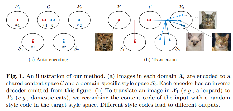
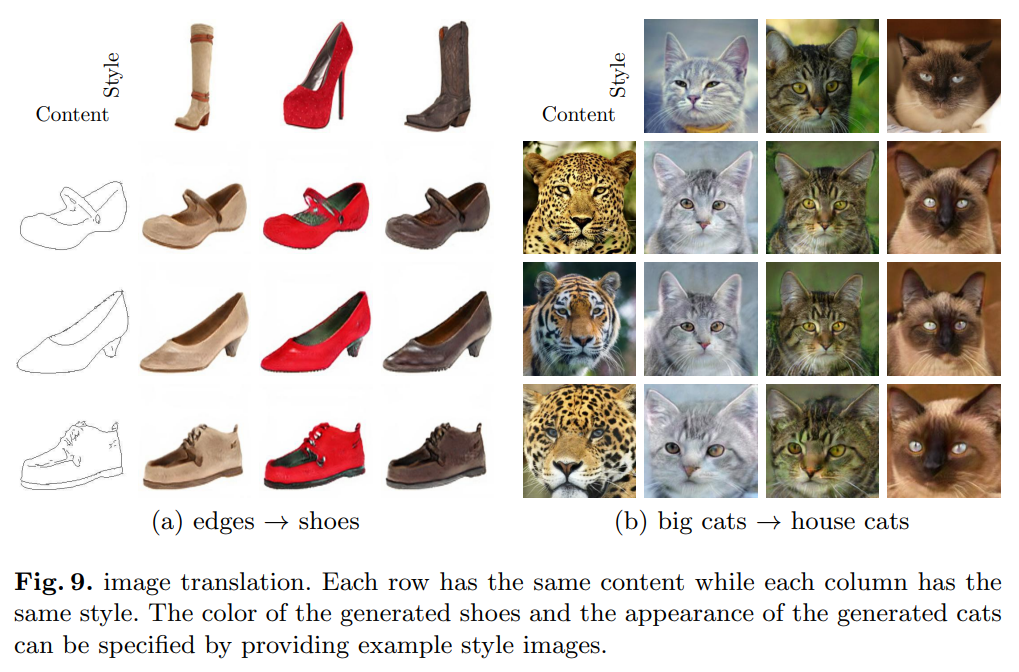
위의 그림은 Multi-Modal Unsupervised Image-to-Image translation의 흐름을 보여준다. 먼저 이미지를 content와 style로 decompose하고, source domain의 content와 target domain의 style을 결합하여 새로운 이미지를 생성해 낼 수 있다.

이 framework에서는 크게 두 가지 가정을 필요로 한다.

1. 한 이미지의 latent space는 content space와 style space로 분해될 수 있다.

2. 서로 다른 domain의 이미지들은 content space를 공유하지만, 각기 다른 style space를 가지고 있다.

여기서 content는 translation에서 보존되어야하는 information, style은 input image에 포함되지 않는 나머지 variation을 의미한다. 논문에서는 content를 underling spatial structure, style을 rendering of the structure라고 표현하고 있다.

2. Multimodal Unsupervised Image-to-Image Translation

2.1 Assumptions

서로 다른 두 도메인 $x_1 \in \mathcal{X}_1, x_2 \in \mathcal{X}_2$가 있다고 하자. unsupervised image-to-image translation에서는 joint distribution $p(x_1, x_2)$에 대한 정보 없이, 각 도메인에 대한 marginal distribtuin $p(x_1), p(x_2)$만 주어진 상황에서, 학습된 image-to-image translation model $p(x_{1 \to 2}|x_1)$과 $p(x_{2 \to 1}|x_2)$를 이용해 두 conditional distribution $p(x_2|x_1)$과 $p(x_1|x_2)$를 estimate하는 것이다. 일반적으로 $p(x_2|x_1)$과 $p(x_1|x_2)$은 complex하고 multimodal distribution을 갖기 때문에 deterministic translation model은 잘 작동하지 못할 가능성이 크다.

이러한 문제를 해결하기 위해 이 논문에서는 partially shared latent space assumption을 제안한다. 이는 각 도메인에서 각 이미지 $x_i \in \mathcal{X}_i$가 모든 도메인에서 공유된 content latent code $c \in \mathcal{C}$와 각 도메인 특정의 style latent code $s_i \in \mathcal{S}_i$로 생성되었다는 가정으로, joint distribution으로부터 상응하는 pair image $(x_1, x_2)$가 $x_1 = G_1^*(c,s_1)$와 $x_2 = G_2^*(c,s_2)$로부터 생성될 수 있다는 의미이다.
또한, generator인 $G_1^*$와 $G_2^*$는 deterministic function이고, 각각 inverse encoder $E_1^* = (G_1^*)^{-1}$와 $E_2^* = (G_2^*)^{-1}$가 있다고 가정한다. 비록 encoder와 decoder가 deterministic function일지라도, $p(x_2|x_1)$은 style $s_2$에 대한 dependency로 인해 contiunous distribution을 가지게 된다. (stochastic mapping)

2.2 Model

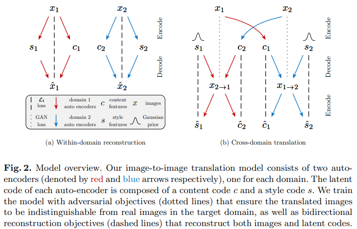
Image-to-Image translation은 CYCLEGAN과 마찬가지로 domain 갯수만큼의 encoder와 decoder로 구성된다.

$x_1 \in \mathcal{X}_1$의 이미지를 $\mathcal{X}_2$로 변환한다고 할 때,
먼저 auto-encoder를 통해 content와 style을 분리하고, $(c_1,s_1) = (E_1^c(x_1),E_1^s(x_1)) = E_1(x_1)$ , $x_1$의 content latent code $c_1$와 prior distribution $q(s_2)\sim\mathcal{N}(0,I)$로부터 추출된 style latent code $s_2$를 이용해 $x_{1\to2} = G_2(c_1,s_2)$를 통해 최종 output image를 생성해 낸다.

2.3 Loss

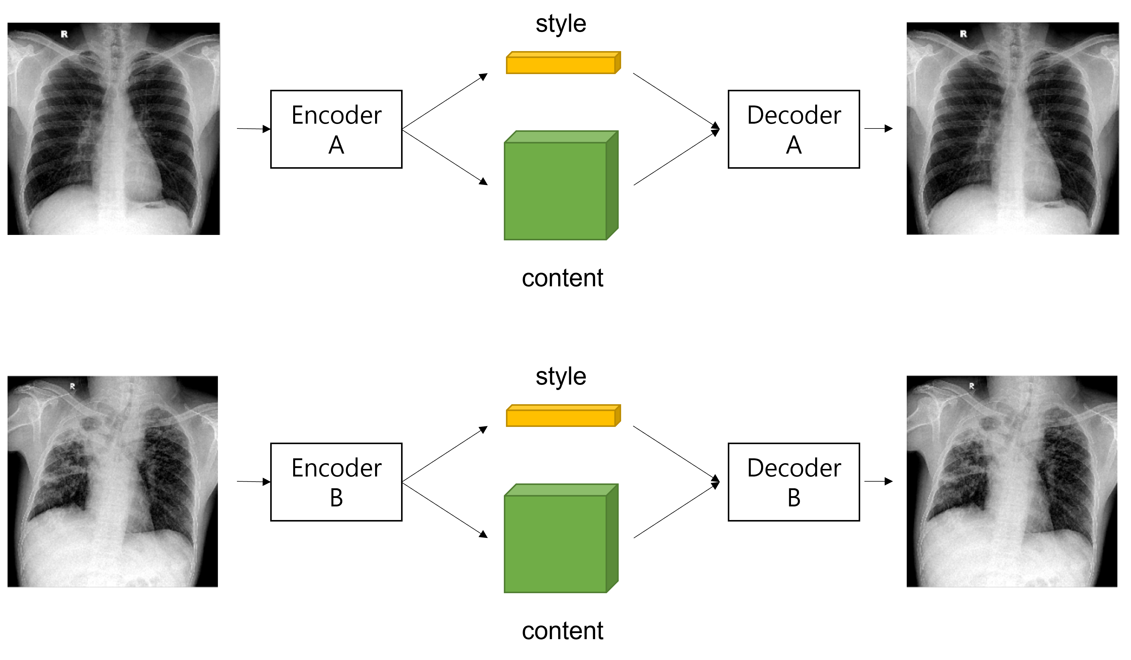
그림 예시는 X-ray로 normal image $\leftrightarrow$ abnormal image로

2.3.1 Bidirectional Reconstruction Loss

(1) Image Reconstruction : data distribution으로부터 추출된 image를 encoding하고 decoding했을 때, 다시 recon이 가능해야한다.

(2)Latent Reconstruction : translation 시, latent distribtion에서 추출된 latent code(style과 content)는 decoding하고, encoding했을 때, 다시 recon이 가능해야 한다.

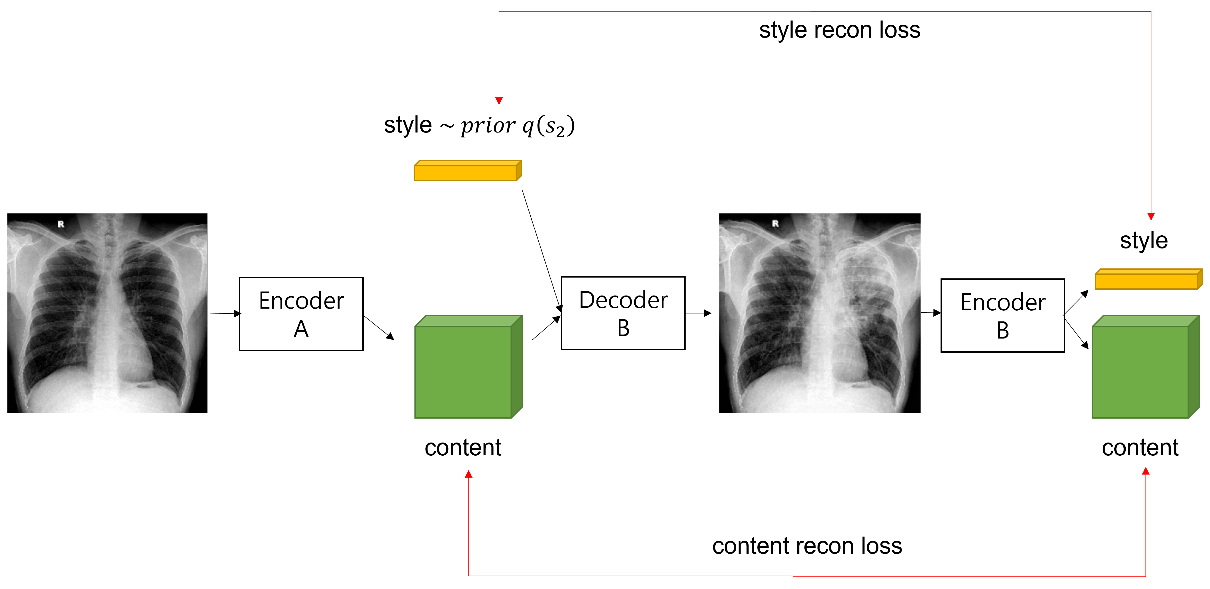
$\mathcal{L}_{recon}^{s_i}$는 서로 다른 style code로 부터 다양한 출력이 나올 수 있도록 해주고, $\mathcal{L}_{recon}^{c_i}$는 변환된 이미지가 원본 이미지의 중요한 content를 유지할 수 있도록 해준다.

2.3.2 Adversarial Loss

translated image의 분포가 target data distribution과 match하게 하기 위해 GAN을 사용한다. 즉, model을 통해 생성된 이미지가 target domain에서의 진짜 이미지와 구분되지 못하게 해야한다.

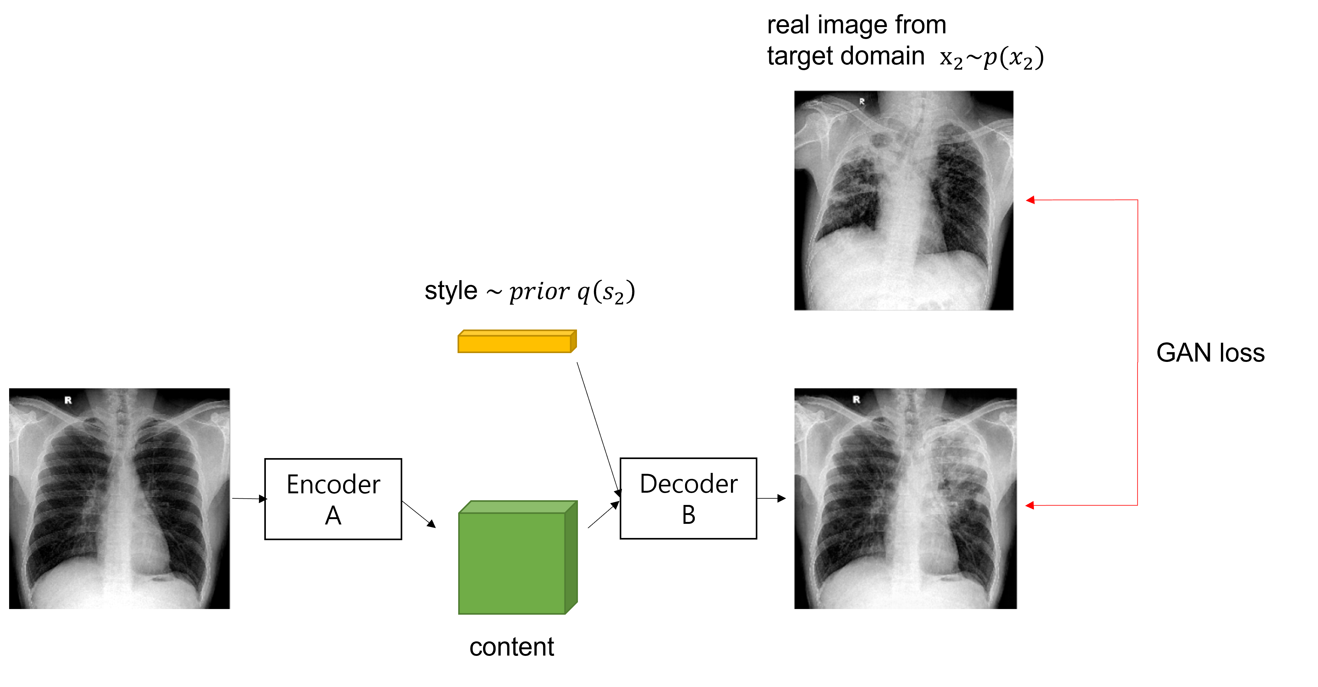
여기서 $D_2$는 discriminator로, $\mathcal{X}_2$의 진짜 이미지와 translated image를 구분하려고 하는 network이다.

2.3.3 Total Loss

결국 최적화하고자 하는 object function은 다음과 같다.

3. Theoretical Analysis

해당 논문에서는 위에서 정의한 loss를 최소화하는 것이 다음의 세 가지 효과를 가져온다고 한다.

(1) Latent Distribution Matching
Image generation task에서 기존의 auto-encoder와 GAN을 결합하는 방법들은 KL divergence나 GAN loss를 이용하여 decoder의 input이 되는 latent distribution과 encode된 latent distribtion을 맞춰주었다. (VAE 정리를 참고)

왜냐하면 decoder가 매번 다른 latent distribution을 받게 되면 auto-encoder training 시 GAN 학습이 잘 될 수 없기 때문이다.

object function에는 명시적으로 이 두 분포를 같게 해주는 term이 없지만, 최종 loss가 minimize된 상황에서 다음의 조건이 만족된다.

위의 명제는 최적점에서 encoding된 style distribution이 gaussian prior와 matching된다는 것을 의미한다. 또한, encoding된 content distribution이 서로 다른 domain에서 encoding된 distribution과 일치한다는 것을 의미한다. $\to$ content space가 domain-invariant

(2) Joint Distribution Matching
우리 모델이 최종적으로 배우고자 하는 것은 두 개의 conditional distribution $p(x_{1\to2}|x_1)$와 $p(x_{2\to1}|x_2)$이고, 각 domain의 data distribution(marginal distribution)을 알면, joint distribution $p(x_{1\to2},x_1)$, $p(x_{2\to1},x_2)$을 정의할 수 있다. (기본 통계 정리 참고)

이 두 joint distribution은 결국 true joint distribution $p(x_1,x_2)$를 추정하기 위한 joint distribution으로, 두 분포가 서로 같아야 이상적이다.

joint distribution matching은 unsupervised image to image translation 문제에서 중요한 constraint이다.

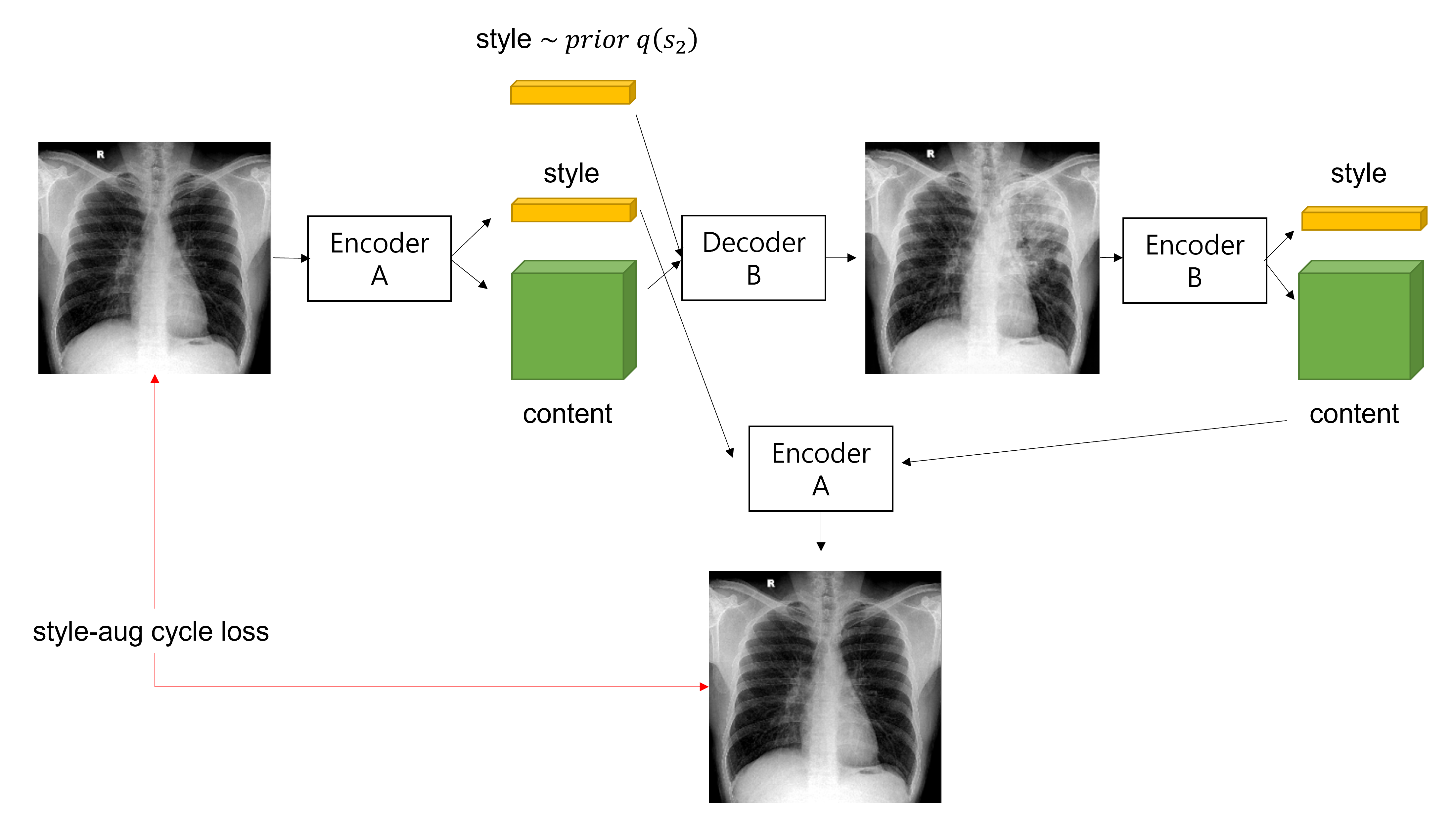
(3) Style Augmented Cycle Consistency
joint distribution matching은 보통 deterministic model과 matched marginal을 가정한 상황에서 cycle consistency constraint를 통해 이루어진다. 하지만 이는 multimodal image translation 문제에서는 너무 강한 constraint이기 때문에 해당 논문에서는 weak form of cycle consistency인 style-augmented cycle consistency를 제안한다.

이는 target domain으로 이미지를 변환시켰다가 다시 original style을 이용하여 original domian으로 변환시켰을 때, original image를 만들어내야 한다는 것을 의미한다. bidirectional reconstruction loss에 그 내용이 포함되어있지만, 몇몇의 경우에서는 명시적으로 cycle loss를 주는 것이 좋다.

4. Implementation

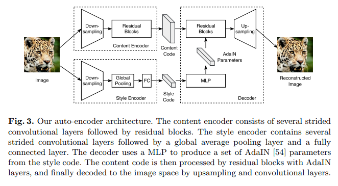
MUNIT network는 Auto-Encoder 구조를 따르고, content encoder, style encoder, 그리고 joint decoder로 이루어져 있다.

(1) Content Encoder

• input을 downsampling하기 위한 strided convolutional layers와 residual blocks로 이루어져 있다.
• 모든 convolutional layers에는 Instance Normalization이 적용된다.

(2) Style Encoder

• strided convolutional layers와 global average pooling layer, 그리고 fully connected layer로 이루어져 있다.
• IN은 중요한 style information을 나타내는 original feature의 mean과 variance를 없애기 때문에 style encoder에는 IN layer를 사용하지 않는다.

(3) Decoder

• residual block을 거친 뒤, upsampling과 convolutional layer를 거쳐 이미지를 recon한다.
• style을 입히기 위해서 affine transformation parameter를 사용하는 normalization layer를 사용하는 Adaptive Instance Normalization (AdaIN)을 residual block에 사용한다.
• 이때 AdaIN의 parameter는 style code로부터 MLP를 거쳐 생성된다.

여기서 z는 이전 layer의 activation이고, $\mu, \sigma$는 각각 channel-wise mean과 standard deviation을 의미한다. 이때, $\gamma$와 $\beta$는 AdaIN의 parameter로 style code가 MLP에 들어감으로써 생성된다.

$\to$ AdaIN의 가장 중요한 포인트는 activation의 affine transformation을 통해 style을 변화시킬 수 있다는 것으로 이해할 수 있다.

(4) Discriminator

• discriminator가 조금 더 높은 scale에서도 잘 작동하도록 3개의 서로 다른 scale에서 작동하는 multi-scale discriminator를 사용한다.
• objective function으로는 LSGAN을 사용한다.

(5) Domain-invariant perceptual loss $\to$ 사용해 볼 만 할 것 같다.

• 보통 perceptual loss는 pair가 있는 경우 output과 reference image 사이에 VGG feature space에서 거리를 loss로 사용하는 것으로, image tranlation에서 효과가 있다고 알려져 있다.
• 하지만, 우리는 unsupervised setting이므로, 이 논문에서는 이를 더욱 domain-invariant하게 만들기 위해 input자체를 reference로 사용한다. 대신, VGG feature distance를 계산하기 전에, Instance Normalization을 사용하여 original feature에서 domain specific한 정보(즉, style)을 담고 있는 mean과 variance를 제거한다.
• 512x512가 넘는 high resolution image에서 효과가 있다고 한다.

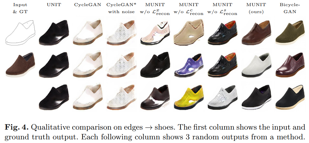
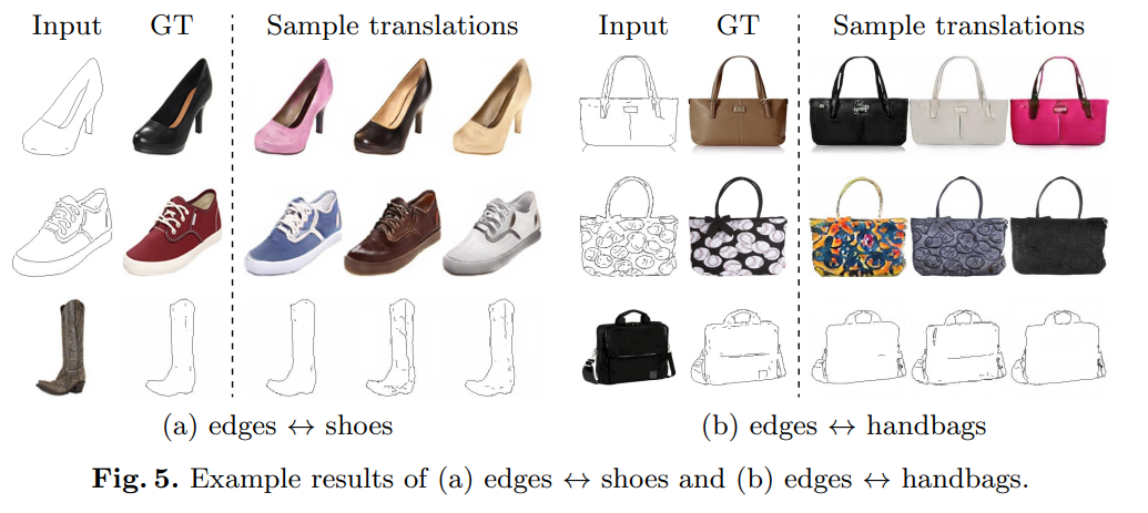
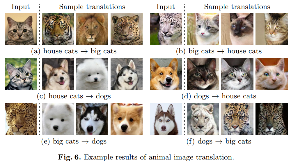
5. Experiments

타 모델보다 좋은 퀄리티로 더 다양한 이미지를 생성할 수 있다고 한다. 또한 내가 원하는 example을 이용하여 content와 style을 결합한 이미지를 생성할 수 있다고 한다. 하지만 이 부분은 아직 부족하다고 생각된다. 조금 더 발전된 논문을 찾아봐야 할 것 같다.

6. Discussion

• multimodal image translation에 대해서 합리적으로 풀어낸 논문 같다
• latent space의 distribution이 generated image space의 distribution과 어떻게 연관이 되는지 눈으로 확인해보고 싶은데, 조금 더 연구가 필요하겠다.