Paper: End-to-End Object Detection with Transformers
Code : github.com
DETR - README
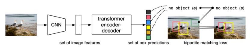
DETR의 핵심적인 마인드는 Object detection task가 "복잡한 라이브러리를 최소화 하고, Classification 처럼 간단하게 행해져야 한다" 는 것입니다. 기존의 Faster R-CNN, YOLO와 같은 전통적인 object detection 모델은 NMS 등 수 많은 proposals을 추려내는 과정을 거쳐야 하지만, 본 연구가 제안하는 모델은 Transformer encoder-decoder와 Bipartite matching을 이용해 유니크한 예측들을 행하는, 아주 간단한 구조로 이루어져 있습니다(아래 그림).
그렇기에, Inference code도 50줄 내외의 짧은 코드로 이루어져 있다고 강조하곤 합니다.
Model Zoo
동물원할 때 Zoo 맞습니다.
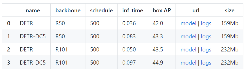
저자들은 우선 Object Detection baseline으로 DETR과 DETR-DC5 모델을 제공합니다. 성능(AP) 은 COCO 2017 val5k을 사용해 평가했으며, 실행 시간(Inference Time) 은 첫 100개의 이미지에 대해 측정됩니다.
또한, Panoptic segmentation 모델도 제공합니다.

Notebooks
저자들은 DETR에 대한 이해를 돕기 위해 colab에서 몇 가지의 notebook을 제공합니다.
DETR's hands on Colab Notebook
해당 Notebook에서는 아래와 같은 요소를 제공합니다.
1. hub에서 모델을 불러오는 방법
2. 예측을 생성하는 방법
3. 모델의 attention을 시각화하는 방법(논문의 figure와 유사)
Standalone Colab Notebook
해당 Notebook에서는 아래와 같은 요소를 제공합니다.
1. 가장 간단한 버전의 DETR을 50 lines of python code로 실행하는 방법
2. 예측을 시각화하는 방법
본 notebook은 DETR의 구조를 이해하는 데 큰 도움이 됩니다. 그렇기에 code를 낱낱이 해부하기 전에 해당 노트북을 먼저 보는 게 좋습니다.
Panoptic Colab Notebook
해당 Notebook은 아래와 같은 요소를 제공합니다.
1. Panoptic segmentation을 위한 DETR을 사용하는 방법
2. 예측을 시각화하는 방법
Usage - Object detection
DETR은 위에서 기술했던 대로 기존의 패키지들에 크게 의존적이지 않습니다. 전반적인 설치 파이프라인은 아래와 같습니다.
- Repository clone:
git clone https://github.com/facebookresearch/detr.git- Install PyTorch 1.5+ and torchvision 0.6+:
conda install -c pytorch pytorch torchvision- Install pycocotools and scipy
conda install cython scipy
pip install -U 'git+https://github.com/cocodataset/cocoapi.git#subdirectory=PythonAPI'
pycocotolls는 COCO dataset에 evaluation을 하기 위한 툴입니다.
. (Panoptic segmentation을 사용하고 싶을 경우) Install panopticapi
pip install git+https://github.com/cocodataset/panopticapi.gitData preparation
본 연구에서 대표적으로 사용한 dataset은 COCO 2017입니다. 주석(annotation)이 포함된 train/val image는 http://cocodataset.org 에서 다운받을 수 있습니다. 해당 dataset의 structure는 아래와 같아야 합니다.
path/to/coco/
  annotations/  # annotation json files
  train2017/    # train images
  val2017/      # val images
Training
예시로 node 당 8 gpus를 사용해 300 epoch을 학습시킬 경우 아래와 같은 명령어를 사용하면 됩니다.
python -m torch.distributed.launch --nproc_per_node=8 --use_env main.py --coco_path /path/to/coco 1 epoch은 28분 정도 걸리기에, 300 epoch은 6일정도 걸릴 수 있습니다(V100 기준).
결과 재생산을 용이하기 하기 위해 저자들은 150 epoch schedule에 대한 results and training logs를 제공합니다(39.5/60.3 AP/AP50).
저자들은 transformer를 학습하는 데 1e-4의 학습률을, backbone을 학습하는데 1e-5의 학습률을 적용한 AdamW을 DETR 학습에 적용합니다. Augmentaiton을 위해 Horizontal flips, scales, crops가 쓰였습니다. 이미지들은 최소 800, 최대 1333의 size를 갖게끔 rescaled됩니다. Transformer는 0.1의 dropout을, 전체 모델은 0.1의 grad clip을 사용해 학습됩니다.
Evaluation
DETR R50을 COCO val5k에 대해 평가하고 싶으면 아래와 같은 명령어를 실행하면 됩니다.
python main.py --batch_size 2 --no_aux_loss --eval --resume https://dl.fbaipublicfiles.com/detr/detr-r50-e632da11.pth --coco_path /path/to/coco모든 DETR detection model에 대한 평가 결과는 제공합니다. (github 방문). 단, GPU 당 batch size(number of images)에 따라 결과가 상당히 변합니다. 예를 들어, batch size 1로 학습한 DC5 모델의 경우 GPU 당 1개 이상의 이미지를 사용해 평가할 경우 성능이 굉장히 낮게 나옵니다.
Usage- Segmentation
본 단락은 Segmentation을 사용하게 될 때 작성할 예정입니다.
Detectron2 wrapper
본 연구는 DETR을 위한 Detectron2 wrapper를 제공함으로써, 기존에 존재하는 detection 방법들과 통합하는 방법을 제시합니다. 이를 통해 Detectorn2에서 제공되는 데이터셋과 backbone 모델을 쉽게 활용할 수 있습니다.
Detectron2란?
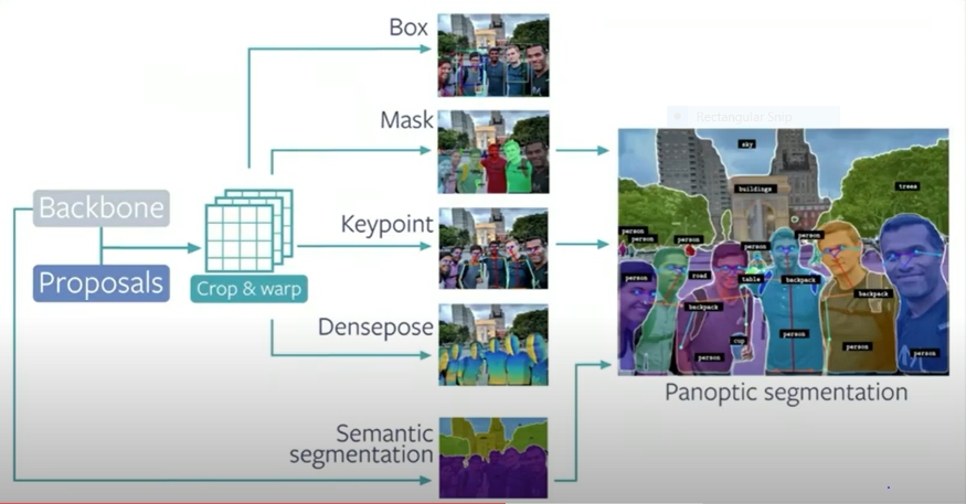
Detectron2는 Facebook에서 개발한, object detection/semantic segmentation을 위한 training/inference 오픈소스입니다. 새로운 task에 fine-tuning하는 과정만 거치면 Detectron을 통해 많은 backbones모델과 dataset을 활용할 수 있게 됩니다.
즉, 단지 새로운 모델만 개발하게 된다면, 기존의 딥러닝 학습과 달리 engine을 이용해 자동화된 학습을 진행할 수 있습니다. CUDA/C Programming을 통해 연산량을 최적화 하기도, object detection에 쓰이는 좋은 학습 기법들에 대한 노하우를 공유해주기도 합니다.
이렇듯, DETR의 저자들은 훌륭한 ObjectDetection-related 모델인 Detectron2를 DETR을 위해 사용하는 CODE를 제공합니다.
물론 아직 Box Detection에 대해서만 활용하고 있다고 합니다.
DETR - Implementation
Import Library
import requests
import matplotlib.pyplot as plt
import time

from PIL import Image
import requests
import matplotlib.pyplot as plt
%config InlineBackend.figure_format = 'retina'

import torch
from torch import nn
from torchvision.models import resnet50
import torchvision.transforms as T
torch.set_grad_enabled(False);
Preprocessing(on COCO dataset)
# COCO classes
CLASSES = [
    'N/A', 'person', 'bicycle', 'car', 'motorcycle', 'airplane', 'bus',
    'train', 'truck', 'boat', 'traffic light', 'fire hydrant', 'N/A',
    'stop sign', 'parking meter', 'bench', 'bird', 'cat', 'dog', 'horse',
    'sheep', 'cow', 'elephant', 'bear', 'zebra', 'giraffe', 'N/A', 'backpack',
    'umbrella', 'N/A', 'N/A', 'handbag', 'tie', 'suitcase', 'frisbee', 'skis',
    'snowboard', 'sports ball', 'kite', 'baseball bat', 'baseball glove',
    'skateboard', 'surfboard', 'tennis racket', 'bottle', 'N/A', 'wine glass',
    'cup', 'fork', 'knife', 'spoon', 'bowl', 'banana', 'apple', 'sandwich',
    'orange', 'broccoli', 'carrot', 'hot dog', 'pizza', 'donut', 'cake',
    'chair', 'couch', 'potted plant', 'bed', 'N/A', 'dining table', 'N/A',
    'N/A', 'toilet', 'N/A', 'tv', 'laptop', 'mouse', 'remote', 'keyboard',
    'cell phone', 'microwave', 'oven', 'toaster', 'sink', 'refrigerator', 'N/A',
    'book', 'clock', 'vase', 'scissors', 'teddy bear', 'hair drier',
    'toothbrush'
]

# colors for visualization
COLORS = [[0.000, 0.447, 0.741], [0.850, 0.325, 0.098], [0.929, 0.694, 0.125],
          [0.494, 0.184, 0.556], [0.466, 0.674, 0.188], [0.301, 0.745, 0.933]]

# standard PyTorch mean-std input image normalization
# 1. 이미지의 높이와 너비 중 작은 사이즈가 800으로 고정됩니다.
# 2. Tensor에 맞게끔 [w,h] format이 [h,w] format으로 변합니다.
# 3. dataset의 mean, std를 이용해 정규화가 진행됩니다. (값이 -3과 3사이에 대부분 분포합니다)
transform= T.Compose([
    T.Resize(800), # * 이유.
    T.ToTensor(),
    T.Normalize([0.485, 0.456, 0.406], [0.229, 0.224, 0.225]) # dataset을 확인하면 된다
])

# output bounding box 후처리
def box_cxcywh_to_xyxy(x):
    x_c, y_c, w, h = x.unbind(1)
    b = [(x_c - 0.5 * w), (y_c - 0.5 * h),
         (x_c + 0.5 * w), (y_c + 0.5 * h)]

    return torch.stack(b, dim=1)

def rescale_bboxes(out_bbox, size):
    img_w, img_h = size
    b = box_cxcywh_to_xyxy(out_bbox)
    b = b * torch.tensor([img_w, img_h, img_w, img_h], dtype=torch.float32)
    return b
Define DETR
class DETRdemo(nn.Module):
    """
    DETR의 demo버전은 아래와 같은 요소가 논문에 쓰인 모델과 다릅니다.
    * learned positional encoding(원래 sine 사용)
    * positional encoding은 input에 pass(원래 attention에 pass)
    * fc bbox predictor (원래 MLP)

    성능은 약 ~40 AP정도 나오며, 1 batch size만 지원한다.
    """

    def __init__(self, num_classes, hidden_dim=256, nheads=8,
                num_encoder_layers=6, num_decoder_layers=6):

        # nn.Module을 initialize 해줍니다.
        super().__init__()


        # Resnet-50 backbone 모델 할당
        self.backbone = resnet50()
        # backbone은 feature map 생성에만 쓰인다(fully connecter layer는 필요 없음).
        del self.backbone.fc


        # resnet50에서 fc-layer를 제거하고 나면 마지막 output의 차원은 (None, 7, 7, 2048) 입니다. (input이 224 x 224일 때)
        # 그렇기에, input channel : 2048, output channel 256(hidden_dim), kernel size 1인
        # conv layer를 추가해줌으로써 channel의 차원을 256로 낮춰줍니다.
        # 여기서 256차원은 transformer의 input tokens의 차원이기도 합니다(token의 length는 가변적입니다).
        self.conv = nn.Conv2d(2048, hidden_dim, 1)

        # pytorch 내 기본 transformer 추가
        self.transformer = nn.Transformer(hidden_dim, nheads,
                                        num_encoder_layers, num_decoder_layers)

        # 예측을 위한 prediction heads에 background detection을 위한 1 extra class를 추가해줍니다.
        # 단, original DETR에서 linear_bbox는 3-layer MLP을 사용합니다.
        self.linear_class = nn.Linear(hidden_dim, num_classes + 1)
        self.linear_bbox = nn.Linear(hidden_dim, 4)

        # output positional encodings(object queries) 추가
        # 100 x 256 차원의 가우시안분포(default)
        # 이 때, 100은 transformer decoder의 sequence입니다.
        self.query_pos = nn.Parameter(torch.rand(100, hidden_dim))

        # spatial positional embeddings
        # 역시, original DETR에서는 sine positional encodings을 사용합니다(demo 버전에선 학습용).
        # 이 때 demo 버전에서는 input의 size를 800 x n 으로 맞춥니다(800<=n<=1600).
        # backbone인 resnet을 통과시키고 나면 size가 32분의 1로 줄기 때문에
        # feature map의 width(또는 height)는 50을 넘지 않습니다.
        # forward 단계에서 각 feature map의 size에 맞게 slicing해 사용하게 됩니다.
        # hidden dimension의

        self.row_embed = nn.Parameter(torch.rand(50, hidden_dim//2))
        self.col_embed = nn.Parameter(torch.rand(50, hidden_dim//2))

    def forward(self, inputs):

        # Resnet-50에서 average pooling layer 전까지 순전파시킵니다.
        # resnet은 최초의 convolution - batch norm - relu - maxpool을 거친 후,
        # conv-batch norm을 주 구성요소로 하는 Bottleneck layer을 굉장히 많이 통과시킵니다.
        x = self.backbone.conv1(inputs)
        x = self.backbone.bn1(x)
        x = self.backbone.relu(x)
        x = self.backbone.maxpool(x)

        x = self.backbone.layer1(x) # layer1은 downsampling을 진행하지 않습니다.
        x = self.backbone.layer2(x)
        x = self.backbone.layer3(x)
        x = self.backbone.layer4(x)
        # avg-layer는 사용하지 않습니다.
        # 여기서 tensor x의 shape은 [None, 2048, input_height//32, input_width//32] 입니다.

        # 2048차원의 channel을 가진 feature map(planes)을 256차원의 channle의 feature map으로 축소시킵니다.
        h = self.conv(x)
        # 여기서 tensor h의 shape은 [None, 256, input_height//32, input_width//32] 입니다.


        # positional encoding을 구성합니다.
        H, W = h.shape[-2:] # backbone + conv를 통해 생성된 feature map의 높이와 너비입니다.

        # 아래의 positional embeddings을 transformer의 input tokens(1d flattened feature map, 즉 tensor h)와 concat함으로써
        # 위치 정보가 없는 input tokens에 위치 정보가 담기게 됩니다.

        # 높이, 너비 각각 feature map의 size에 해당하는 positional embeddings을 slicing합니다.
        # column 정보를 담은 positional embeddings (H x W x 128)과 --> H는 그저 차원을 맞추기 위함입니다.
        # row 정보를 담은 positional embeddings (H x W x 128)를 생성한 후 --> W는 그저 차원을 맞추기 위함입니다.
        # concat을 시켜 transformer의 input tokens의 차원인 256과 일치시킨 후
        # (H x W x 256)의 2d positional embeddings을 (HW x 256)의 1d positional embeddings으로 flatten 해줍니다.

        # 이는 2d feature map이 transformer의 input tokens으로 쓰이기 전에 1d feature sequence로 flatten 하는 것과 일치합니다.
        pos=torch.cat([
            self.col_embed[:W].unsqueeze(0).repeat(H, 1, 1),
            self.row_embed[:H].unsqueeze(1).repeat(1, W, 1),
        ], dim=-1).flatten(0, 1).unsqueeze(1)

        # transformer를 순전파시킵니다.
        # 1d feature sequence와 positional embeddings가 concat되어 transformer의 input tokens으로 쓰이고,
        # object queries의 길이에 해당하는 output token을 반환합니다.
        h = self.transformer(pos+0.1*h.flatten(2).permute(2, 0, 1),
                            self.query_pos.unsqueeze(1)).transpose(0,1)

        # 최종적으로, transformer output을 class label과 bounding boxes로 사영시킵니다.
        # 결과의 차원은 (1, len of object queries, # of classes (or 4 in bboxes))입니다.
        return {'pred_logits': self.linear_class(h),
                'pred_boxes': self.linear_bbox(h).sigmoid()}
Import model of pre-trained DETR
detr = DETRdemo(num_classes=91)
state_dict = torch.hub.load_state_dict_from_url(
    url='https://dl.fbaipublicfiles.com/detr/detr_demo-da2a99e9.pth',
    map_location='cpu', check_hash=True)
detr.load_state_dict(state_dict)
detr.eval();
Object detect & visualize
#detect
def detect(im, model, transform):

    # input image를 정규화해줍니다. (batch-size : 1)
    img = transform(im).unsqueeze(0)

    # demo의 경우 aspect ratio를 0.5와 2사이만 지원합니다.
    # 이 범위 밖의 이미지를 사용하고 싶다면 maximum size을 1333이하로 rescaling해야 합니다.
    assert img.shape[-2] <= 1600 and img.shape[-1] <= 1600

    # model을 통과시킵니다.
    outputs = model(img)

    # 70 % 이상의 정확도를 가진 예측만 남깁니다.
    probas = outputs['pred_logits'].softmax(-1)[0, :, :-1]
    keep = probas.max(-1).values > 0.7

    # 0과 1사이의 boxes 값을 image scale로 확대합니다.
    bboxes_scaled = rescale_bboxes(outputs['pred_boxes'][0, keep], im.size)
    return probas[keep], bboxes_scaled

#visualize
def plot_results(pil_img, prob, boxes):
    plt.figure(figsize=(16,10))
    plt.imshow(pil_img)
    ax = plt.gca()
    for p, (xmin, ymin, xmax, ymax), c in zip(prob, boxes.tolist(), COLORS * 100):
        ax.add_patch(plt.Rectangle((xmin, ymin), xmax - xmin, ymax - ymin,
                                   fill=False, color=c, linewidth=3))
        cl = p.argmax()
        text = f'{CLASSES[cl]}: {p[cl]:0.2f}'
        ax.text(xmin, ymin, text, fontsize=15,
                bbox=dict(facecolor='yellow', alpha=0.5))
    plt.axis('off')
    plt.show()
실행
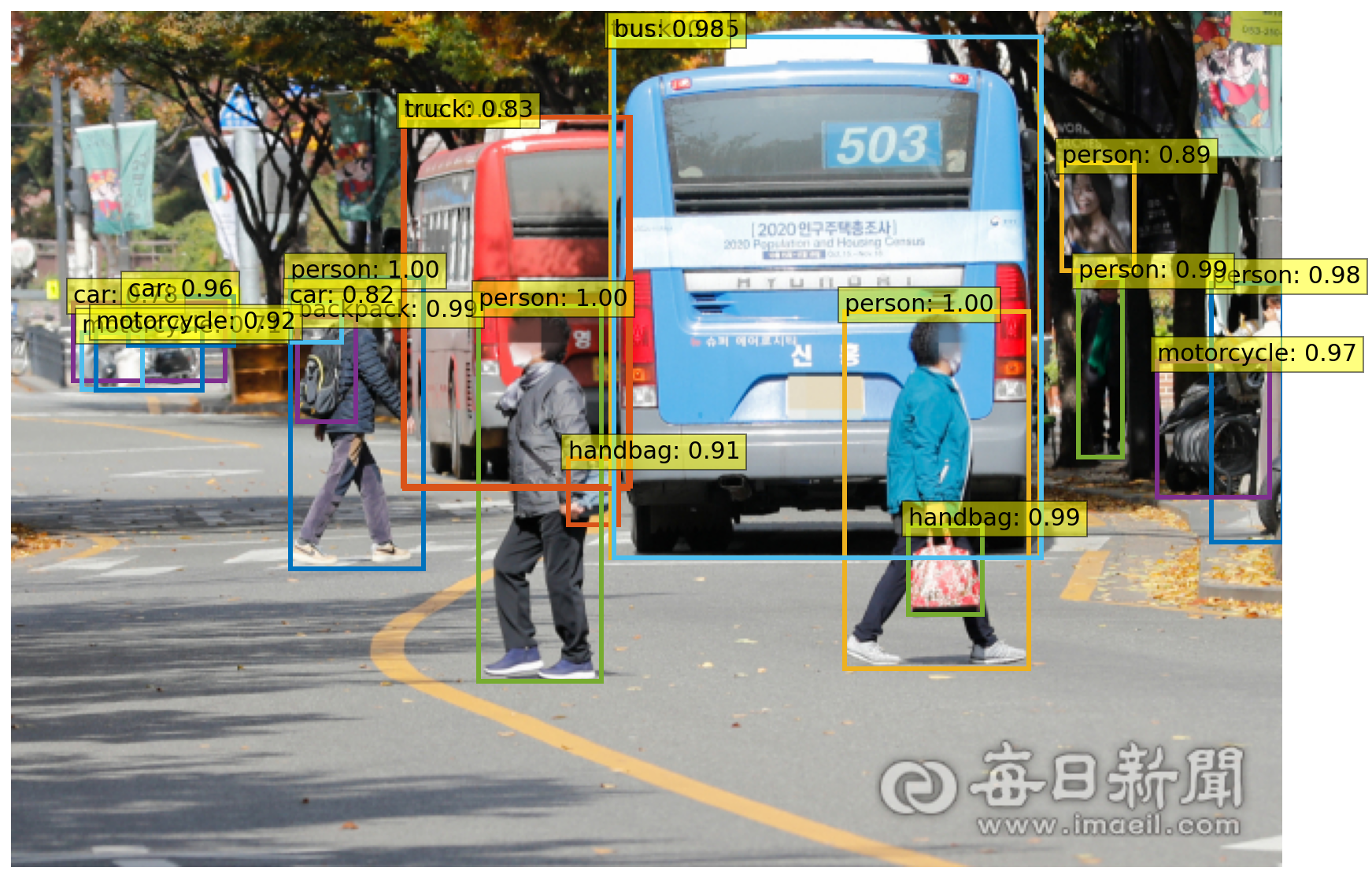
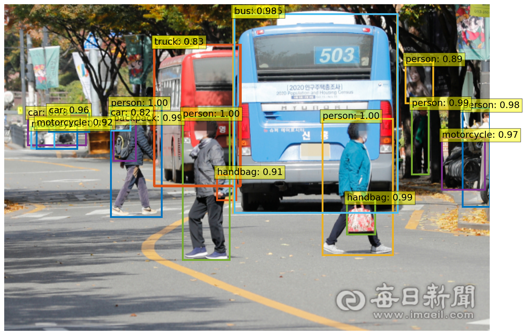
url = 'https://news.imaeil.com/inc/photos/2020/11/02/2020110216374231552_l.jpg'
im = Image.open(requests.get(url, stream=True).raw)

start = time.time()

#Detect
scores, boxes = detect(im, detr, transform)

print("Inference time :", round(time.time()-start, 3), 'sec')
Inference time : 1.1 sec
결과
plot_results(im, scores, boxes)
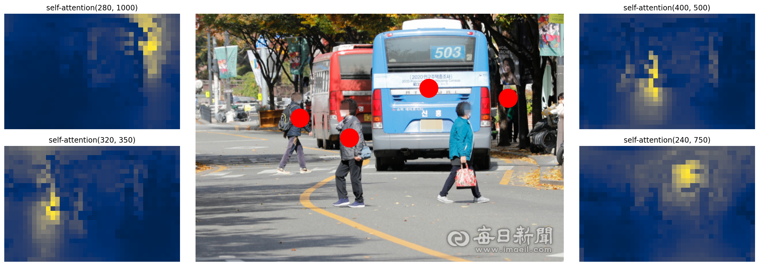
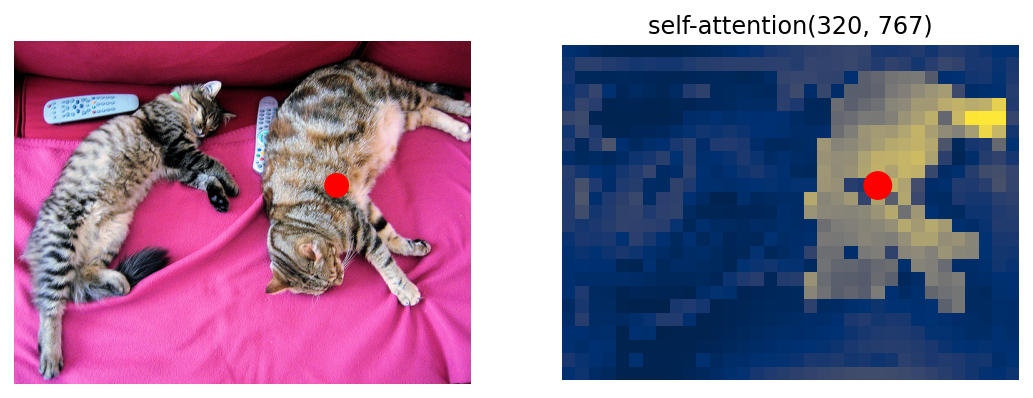
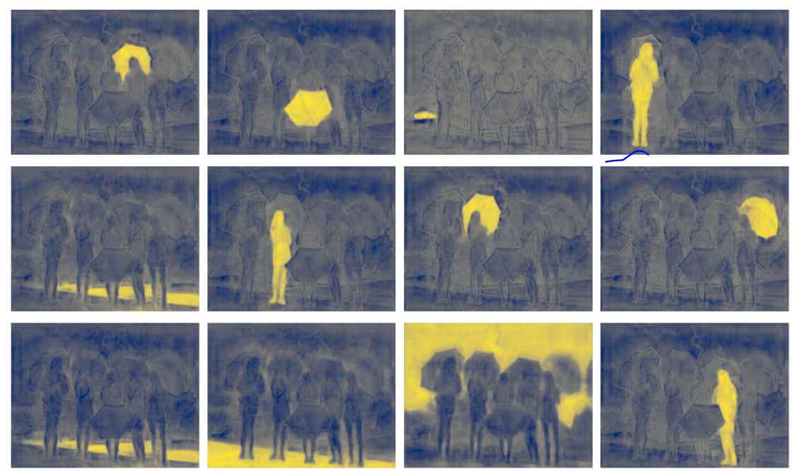
Attention map 시각화 in object detection
코드는
https://github.com/sjinu96/xod/blob/main/DETR_Inference.ipynb
참고하시길 바랍니다.
Encoder-Decoder Cross-attention
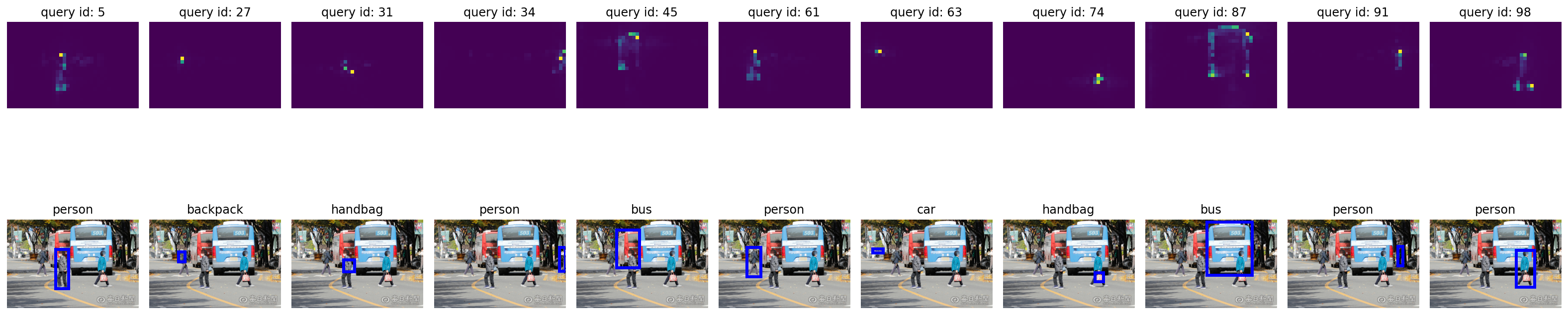
Encoder self-attention