교차 검증과 하이퍼 파라미터 튜닝에 있어서의 내 오해

교차 검증(Cross Validation, CV)은 모델 오버피팅 체크하고 성능 평가할 때 사용됨

근데 난 계속 이것이 궁금했음

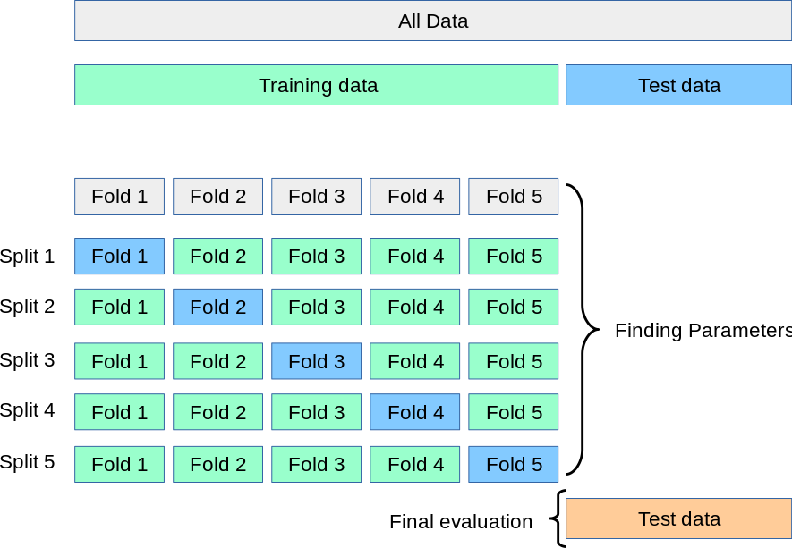
K-fold CV는 데이터를 무작위로 K개의 fold로 나누고 K번 학습하고 검증과정을 거치는 거라고 알고 있는데,
위의 그림에서 전체 훈련셋을 K개의 split으로 나누고, 각 split을 K개의 fold로 나누는 건지
or
전체 훈련셋을 K개의 fold로 나누는게 끝인지

그런데 두번째가 맞다고 함

다시 말하자면, 전체 훈련셋을 K개의 fold로 나눈 후, fold1부터 fold K까지 돌아가며 validation set의 역할을 한다는 것!
(= 각 split은 어느 fold를 validation 용으로 사용하냐의 차이였던 것)

여기서 이 cv를 통해 모델의 정확도는

각 split의 정확도를 구한 후, 만약 정확도의 분산이 크지 않다면
(gpt 피셜 0.05 미만 best, 적어도 0.1 미만)
이 정확도의 평균값을 대표 정확도로 친다.

요렇다고 함

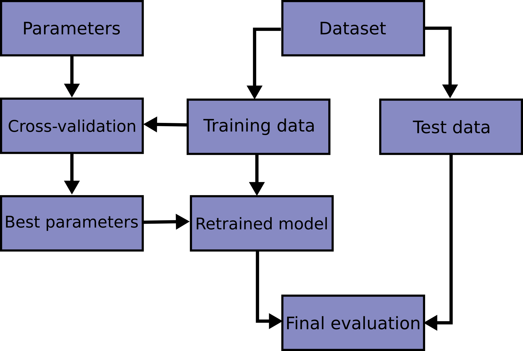
다음으로는 이런 cv를 사용한 하이퍼 파라미터 튜닝 과정을 살펴보자! (GridSearchCV 사용)

여기서는 데이터를 5 folds로 나누고, (5-fold cv)
하나의 하이퍼 파라미터 조합을 사용해 전체 split에 걸쳐 모델을 학습 및 평가함
그러면 그 fold 수 만큼의 accuracy가 산출되는데, 이걸 평균내어 해당 하이퍼 파라미터 조합의 성능을 파악함
그리고 다음 하이퍼 파라미터 조합으로 넘어가 위의 단계를 반복
모든 하이퍼 파라미터 조합에 대한 평가가 끝나면, 성능이 가장 좋은 하이퍼 파라미터 조합을 선택할 수 있음
(즉, 각 하이퍼 파라미터 조합으로 하나의 split이 아닌 모든 split을 다 학습한다는 뜻)

import pprint
from sklearn.model_selection import GridSearchCV

params = {'max_depth' : [2, 4, 7, 10]} # `params` 딕셔너리 정의
wine_tree = DecisionTreeClassifier(random_state=13) # 모델 인스턴스 생성

gridsearch = GridSearchCV(estimator=wine_tree, param_grid=params, cv=5) # GridSearchCV 인스턴스 생성
gridsearch.fit(X, y)

pp = pprint.PrettyPrinter(indent=4)
pp.pprint(gridsearch.cv_results_)

결과)

{   'mean_fit_time': array([0.00809431, 0.01312385, 0.02575712, 0.03695736]),
    'mean_score_time': array([0.0016345 , 0.        , 0.00192189, 0.00371246]),
    'mean_test_score': array([0.6888005 , 0.66356523, 0.65340854, 0.64401587]),
    'param_max_depth': masked_array(data=[2, 4, 7, 10],
             mask=[False, False, False, False],
       fill_value='?',
            dtype=object),
    'params': [   {'max_depth': 2},
                  {'max_depth': 4},
                  {'max_depth': 7},
                  {'max_depth': 10}],
    'rank_test_score': array([1, 2, 3, 4]),
    'split0_test_score': array([0.55230769, 0.51230769, 0.50846154, 0.51615385]),
    'split1_test_score': array([0.68846154, 0.63153846, 0.60307692, 0.60076923]),
    'split2_test_score': array([0.71439569, 0.72363356, 0.68360277, 0.66743649]),
    'split3_test_score': array([0.73210162, 0.73210162, 0.73672055, 0.71054657]),
    'split4_test_score': array([0.75673595, 0.7182448 , 0.73518091, 0.72517321]),
    'std_fit_time': array([0.00507212, 0.00374958, 0.00253127, 0.00350123]),
    'std_score_time': array([0.003269  , 0.        , 0.003101  , 0.00365362]),
    'std_test_score': array([0.07179934, 0.08390453, 0.08727223, 0.07717557])}

# 첫번째 하이퍼 파라미터 조합의 모델을 각 split을 사용해 학습한 후 평가 결과
np.mean([0.55230769, 0.68846154, 0.71439569, 0.73210162, 0.75673595])

결과)

0.688800498

최적의 성능을 나타내는 하이퍼 파라미터는?

print(gridsearch.best_estimator_)
print(gridsearch.best_score_)
print(gridsearch.best_params_)

결과)

DecisionTreeClassifier
DecisionTreeClassifier(max_depth=2, random_state=13)
0.6888004974240539
{'max_depth': 2}

max_depth가 2일 때 모델 성능이 낫다는 결과임

번외) 파이프라인을 적용한 모델에 그리드 서치를 적용하기

from sklearn.pipeline import Pipeline
from sklearn.preprocessing import StandardScaler

estimators = [('scaler', StandardScaler()), # 데이터 전처리(scaling)
              ('clf', DecisionTreeClassifier(random_state=13))] # 모델 생성

pipe = Pipeline(estimators) # 파이프라인 객체 생성

# pipeline을 활용하며 params 하이퍼파라미터들 목록 설정 ('clf__'만 추가된 것)
param_grid = [ {'clf__max_depth': [2, 4, 7, 10]}] 

GridSearch = GridSearchCV(estimator=pipe, param_grid=param_grid, cv=5)
GridSearch.fit(X, y)

print(GridSearch.best_score_)
print(GridSearch.best_params_)

결과)

0.6888004974240539
{'clf__max_depth': 2}

트리 시각화

from graphviz import Source
from sklearn.tree import export_graphviz

# # 기본 방식 트리 시각화
# Source(export_graphviz(wine_tree, feature_names=X_train.columns, # estimator = 트리 인스턴스 자체
#                        class_names=['W', 'R'],
#                        rounded=True, filled=True))

# # 파이프라인 사용한 트리 시각화
# Source(export_graphviz(pipe['clf'], feature_names=X.columns, # estimator = 파이프라인에서 할당한 모델(clf)
#                        class_names=['W', 'R'],
#                        rounded=True, filled=True))

# 파이프라인 + 그리드서치 사용한 트리 시각화
# estimator = 그리드서치에서 찾은 최적의 모델에서 최종의 모델로 지정된 트리 인스턴스)
Source(export_graphviz(GridSearch.best_estimator_['clf'], feature_names=X.columns,
                       class_names=['W', 'R'],    
                       rounded=True, filled=True))

테이블로 하이퍼 파라미터 조합별 모델 성능 확인

score_df = pd.DataFrame(GridSearch.cv_results_)
score_df[['params', 'rank_test_score', 'mean_test_score', 'std_test_score']]

결과)

params	rank_test_score	mean_test_score	std_test_score
0	{'clf__max_depth': 2}	1	0.688800	0.071799
1	{'clf__max_depth': 4}	2	0.663565	0.083905
2	{'clf__max_depth': 7}	3	0.653408	0.086993
3	{'clf__max_depth': 10}	4	0.644016	0.076915

아, 그리고 holdout과 train_test_split()의 차이가 뭔가 했음
둘 다 전체 데이터셋을 훈련셋과 테스트셋으로 한 번 나누는 거니까..
알아보니 holdout을 train_test_split()으로 구현하는 거였음 꺄륵꺄륵