[Image classification] AlexNet
처음으로 벨로그 글을 쓰게 되었습니다. 많이 부족하고 서툴겠지만 좋게 봐주시면 감사하겠습니다.😊
이번에 리뷰하게 된 논문은 ImageNet Classification with Deep Convolutional Neural Networks 입니다.
이 논문은 2012년에 발표된 논문으로써 ImageNet LSVRC에서 우승한 모델을 발표한 논문입니다. 그 모델의 이름은 AlexNet으로 Alex Krizhevsky의 이름을 따서 지어지게 되었습니다. 이 모델은 이미지 분류(Image Classification) 분야에서 큰 성장을 할 수 있게 해주었습니다. 2012년도 대회에서 Top-5 error rate 15.4% 로 26.2%를 기록한 2위(SVM + HoG 모델)와의 큰 차이를 보이며 우승을 하였습니다. AlexNet이 어떻게 이렇게 높은 성능을 낼 수 있었는지 알아보겠습니다🔍
설명 순서
- ImageNet Dataset
- Data Preprocessing
- AlexNet Architecture
- More about AlexNet (Activation ,dropout, pooling, ...)
- AlexNet with Tensorflow code
ImageNet Dataset
우선 ImageNet 데이터에 대해서 설명해보겠습니다. ImageNet 데이터는 22,000 개의 카테고리로 구성되었으며, 1500만장의 고해상도 이미지를 포함하고 있습니다. 또한 LSVRC 대회에서는 ImageNet Dataset의 subset을 통해서 대회를 진행합니다. subset은 1000개의 카테고리를 사용하며 각 카테고리별 1000개의 이미지가 존재합니다.
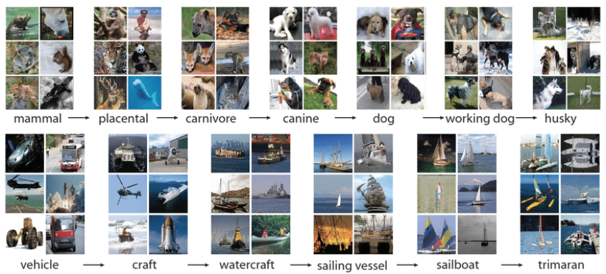 그림1. ImageNet Dataset
Data preprocessing
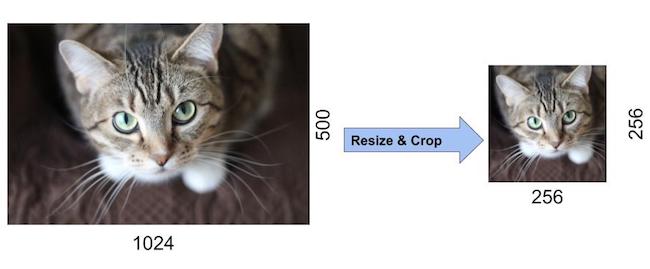
- 이미지의 크기를 고정
이미지를 256x256의 사이즈로 고정하였습니다. 나중에는 FC layer(Fully Connective layer)의 입력 크기가 고정되어야 하기위한 이유입니다. 만약 입력이미지의 크기가 다르게 된다면 FC layer에 입력되는 feature의 개수가 모두 다르게 된다는 문제가 있습니다. 그렇다면 이미지 크기를 고정하는 방법은 무엇이 있을까요? - crop
resize의 방법중 하나로 이미지를 크기에 맞게 잘라주는 방법입니다. AlexNet에서는 resize방법으로 crop을 사용하였습니다. 구체적으로 살펴보자면 이미지의 넓이(width)와 높이(height) 중 더 짧은 쪽을 256으로 고정시켜주었고, 중앙부분은 256x256 크기로 crop 했습니다.
- normalize
각 이미지의 픽셀(pixel)에서 training set의 평균을 빼서 normalize 해주었습니다.
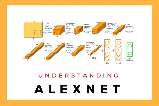
AlexNet Architecture
 그림2. AlexNet Architecture
AlexNet의 구조 특징
- 8개의 레이어로 구성(5개의 Convolution Layer와 3개의 Full-Connected Layer)
- Input Layer -> Conv1 -> MaxPool1 -> Norm1 -> Conv2 -> MaxPool2-> Norm2 -> Conv3 -> Conv4 -> Conv5 ->MaxPool3 -> FC1 -> FC2 -> Output Layer
Input Layer
우선 AlexNet에 입력되는 것은 227x227x3의 이미지이다. (227 pixel x 227 pixel x 3(Red, Blue , Green))
위의 이미지에선 224로 되어있지만 227가 올바른 크기의 사이즈 입니다.
첫번째 레이어(Conv1)
96개의 11 x 11 x 3 사이즈의 필터 커널로 입력된 이미지를 Convolution 하게 됩니다. Convolution의 Stride는 4로 설정되었고 zero-padding은 사용하지 않았습니다. zero-padding은 Convolution 으로 인해 피처맵의 사이즈가 축소되는 것을 방지하기 위해, 또는 축소되는 정도를 줄이기 위해 이미지의 가장자리 부분에 0을 추가하는 것입니다. 결과적으로 55 x 55 x 96 피처맵(96장의 55 x 55 사이즈 특성맵들)이 산출된다. 그 다음에 ReLU 함수로 activation 해줍니다. 추가적으로 input 과 output의 사이즈를 계산하는 방법에 대해서는 https://bskyvision.com/420 에서 자세히 볼 수 있으니 참고바랍니다.
- input : 227x 227 x 3
- output: 55 x 55 x 96
MaxPool1(Conv1)
이어서 3 x 3 overlapping max pooling이 stride 2로 시행됩니다. 그 결과 27 x 27 x 96 피처맵을 갖게 된다.
- input:55 x 55 x 96
- output: 27 x 27 x 96
Norm1(Conv1)
local response normalization이 시행됩니다. local response normalization은 특성맵의 차원을 변화시키지 않으므로, 특성맵의 크기는 27 x 27 x 96으로 유지된다.
- input:27 x 27 x 96
- output: 27 x 27 x 96
Conv2(Conv1)
256개의 5 x 5 x 48 커널을 사용하여 전 단계의 피처맵을 Convolution해줍니다. stride는 1로, zero-padding은 2로 설정했습니다. 따라서 27 x 27 x 256 피처맵(256장의 27 x 27 사이즈 퍼처맵들)을 얻게 됩니다. Conv1과 마찬가지로 ReLU 함수로 Activation합니다.
- input:27 x 27 x 96
- output: 27 x 27 x 256
MaxPool2(Conv1)
그 다음에 3 x 3 overlapping max pooling을 stride 2로 시행합니다. 그 결과 13 x 13 x 256 피처맵을 얻게 됩니다.
- input:27 x 27 x 256
- output: 13 x 13 x 256
Norm1(Conv1)
그 후 local response normalization이 시행되고, 피처맵의 크기는 13 x 13 x 256으로 그대로 유지된다.
- input: 13 x 13 x 256
- output: 13 x 13 x 256
Conv3(Conv1)
384개의 3 x 3 x 256 커널을 사용하여 전 단계의 피처맵을 Convolution해줍니다. stride와 , zero-padding은 1로 설정했습니다. 따라서 13 x 13 x 384 피처맵(384장의 13 x 13 사이즈 퍼처맵들)을 얻게 됩니다. 다른 Conv와 마찬가지로 ReLU 함수로 Activation합니다.
- input: 13 x 13 x 256
- output: 13 x 13 x 384
Conv4(Conv1)
384개의 3 x 3 x 192 커널을 사용하여 전 단계의 피처맵을 Convolution해줍니다. stride와 , zero-padding은 1로 설정했습니다. 따라서 13 x 13 x 384 피처맵(384장의 13 x 13 사이즈 퍼처맵들)을 얻게 됩니다. 다른 Conv와 마찬가지로 ReLU 함수로 Activation합니다.
- input: 13 x 13 x 384
- output: 13 x 13 x 384
Conv5(Conv1)
256개의 3 x 3 x 192 커널을 사용하여 전 단계의 피처맵을 Convolution해줍니다. stride와 , zero-padding은 1로 설정했습니다. 따라서 13 x 13 x 384 피처맵(384장의 13 x 13 사이즈 퍼처맵들)을 얻게 됩니다. 다른 Conv와 마찬가지로 ReLU 함수로 Activation합니다.
- input: 13 x 13 x 384
- output: 13 x 13 x 256
MaxPool3(Conv1)
그 다음에 3 x 3 overlapping max pooling을 stride 2로 시행합니다. 그 결과 6 x 6 x 256 피처맵을 얻게 됩니다.
- input: 13 x 13 x 256
- output: 6 x 6 x 256
FC1(Conv1)
6 x 6 x 256 피처맵을 flatten해줘서 6 x 6 x 256 = 9216차원의 벡터로 만들어줍니다. 그것을 여섯번째 레이어의 4096개의 뉴런과 Fully Connected 해줍니다. 그 결과를 ReLU 함수로 Activation합니다.
- input: 6 x 6 x 256
- output: 4096
FC2(Conv1)
4096개의 뉴런으로 구성되어 있습니다. 전 단계의 4096개 뉴런과 Fully Connected되어 있다. 출력 값은 ReLU 함수로 Activation됩니다.
- input: 4096
- output: 4096
Output Layer(Conv1)
1000개의 뉴런으로 구성되어 있습니다. 전 단계의 4096개 뉴런과 Fully Connected되어 있습니다. 1000개 뉴런의 출력값에 softmax 함수를 적용해 1000개 클래스 각각에 속할 확률을 나타냅니다.
- input: 4096
- output: 1000
More about AlexNet
이 부분에서는 AlexNet에서 사용된 주요 기법에 대해서 알아보겠습니다.
ReLU non-Linearity
ReLU라는 함수를 활용하면 기존 tanh(x) / sigmoid 함수의 saturating non-linearlities의 문제를 해결할 수 있습니다. 처리시간도 감소하였고(논문에 따르면 5~6배), error rate를 감소시키는 데에 걸린 시간도 줄어들었습니다. ReLU함수의 식은 max(0,x)이며, 그 개형은 아래에 있습니다.
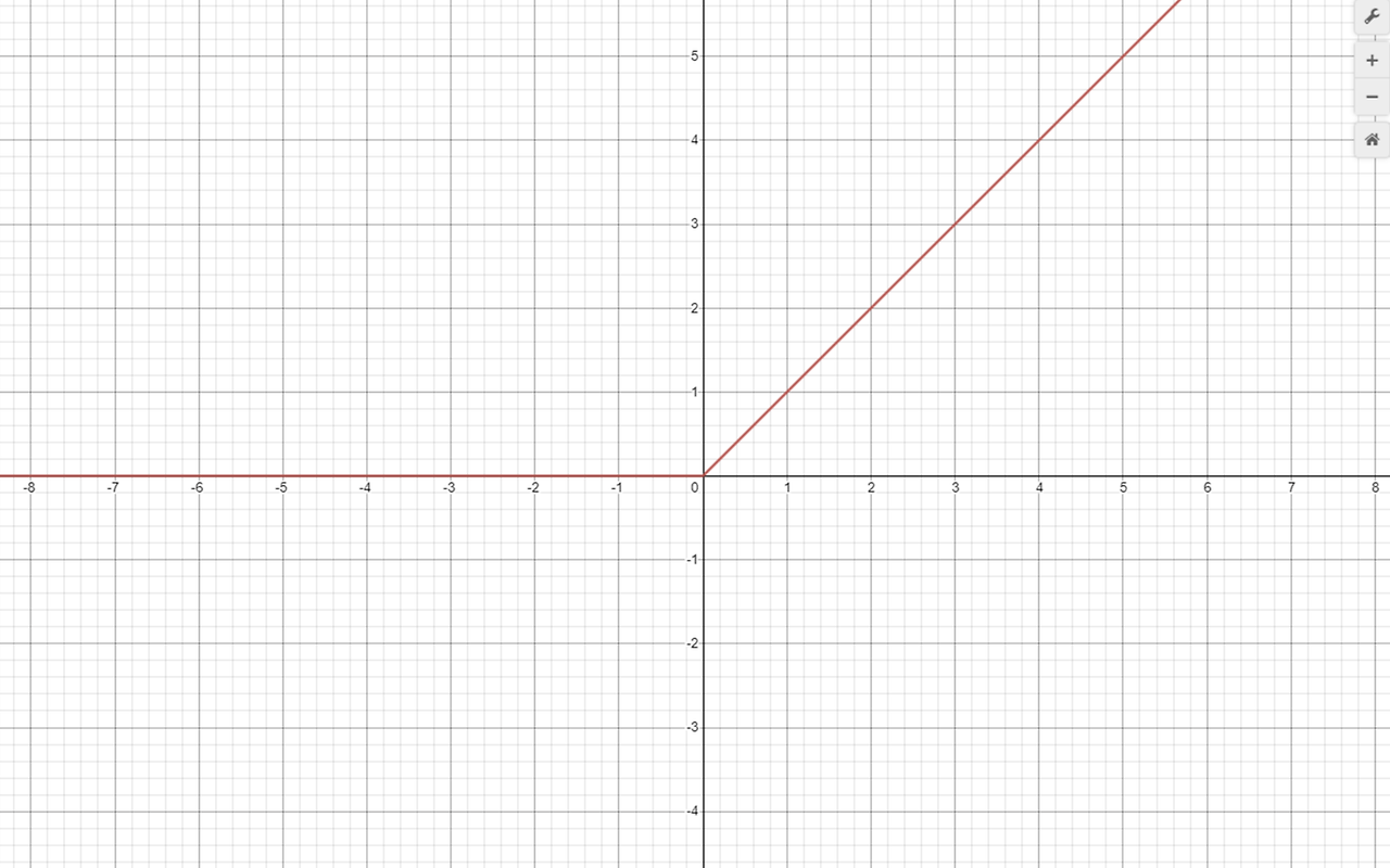
그림3. ReLU
정의역이 0 미만이면 0을 출력하고 , 그 이외의 경우에는 정의역의 수(y=x)를 그대로 출력하며 미분을 할 경우에도 계산이 매우 빠르게 가능하게 한다.
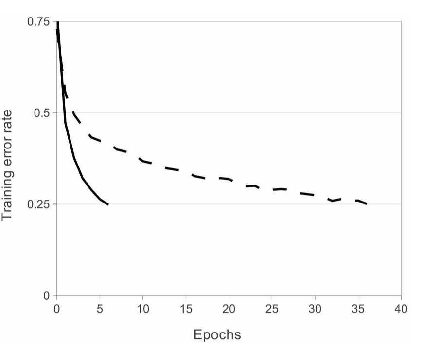
그림4.
ReLU를 사용할 경우 적은 Epoch를 사용하더라도 training error rate가 빠르게 감소하는것을 볼 수 있다.
Multiple GPU
AlexNet에서는 GPU의 한계를 극복하기 위해 2개의 GPU를 사용하였습니다. 이 때 모든 neuron들은 2개의 GPU에 분산되어 있습니다. 그리고 특정 층에서만 소통을 하고, 그 외의 층에서는 각자의 연산을 진행합니다(완벽한 분산). GPU를 여러 개 사용함으로 인해서 처리 시간도 감소하고, error rate도 줄어드는 것을 확인할 수 있습니다. 또한 각각의 GPU는 특정 분야에 특화 되어있음을 확인할 수 있습니다. 예를 들어 첫 번째 GPU는 color-agnostic적인 면을 처리할 수 있고, 두 번째 GPU는 color-specific한 면을 처리할 수도 있습니다.
Local Response Localization (LRN)
LRN은 generalizaion을 목적으로 합니다. sigmoid나 tanh 함수는 입력 data의 속성이 서로 편차가 심하면 saturating되는 현상이 심해져 vanishing gradient(층이 깊어질 수록 값이 작아져 값이 소실됨)를 유발할 수 있게 됩니다. 반면에 ReLU는 non-saturating nonlinearity 함수이기 때문에 saturating을 예방하기 위한 입력 normalizaion이 필요로 하지 않는 성질을 갖고 있습니다. ReLU는 양수값을 받으면 그 값을 그대로 neuron에 전달하기 때문에 너무 큰 값이 전달되어 주변의 낮은 값이 neuron에 전달되는 것을 막을 수 있습니다. 이것을 예방하기 위한 normalization이 LRN 입니다.
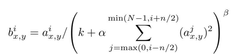
그림5. LRN 수식
Overlapping Pooling
논문에서는 Overlapping Pooling을 통해서 overfitting을 방지하고 top-1 error 와 top-5 error를 각각 0.4% , 0.3%를 낮추었습니다. Pooling layer는 동일한 커널맵에 있는 인접한 neuron의 output을 요약해줍니다. 전통적으로 Pooling Layer에서는 Overlap은 하지않았지만 AlexNet에서는 Overlap을 해주었고 , kernel size =3 , stride=2 로 하여 Overlap하였습니다.
Dropout
Dropout은 신경망의 뉴런을 부분적으로 생략하여 모델의 과적합(overfitting)을 해결해주기 위한 방법중 하나입니다. Dropout은 전체 weight를 계산에 참여시키는 것이 아닐 layer에 포함된 weight 중에서 일부만 참여시키는 것입니다. 여기서 일부만 참여시키는 것이라는 나머지를 제외 시키라는 말이 아니라 나머지 뉴런을 0으로 만드는 것을 의미합니다.
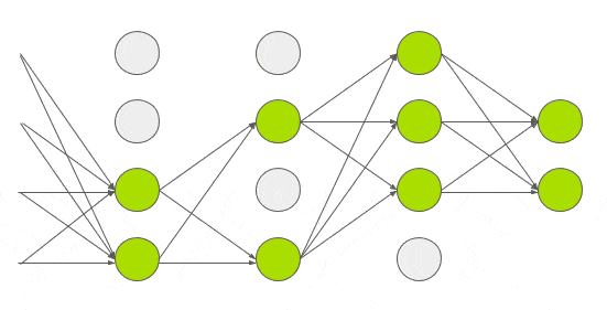
그림6. Dropout
Data Augmentation
Data Augmentation은 CPU를 통하여 진행하였기 때문에 GPU의 계산비용을 방해하지 않는다는 장점이 있습니다. 해당 방법은 크게 image translation & horizontal reflection과 altering intensities of RGB channels in training images로 분류할 수 있습니다.
먼저 Image translation & horizontal reflection 같은 경우, 기존 256*256 픽셀 이미지에서 랜덤하게 224*224 patch와 그것을 가로로 좌우반전한 patch를 추출합니다. 무작위로 픽셀을 선정함으로써 overfitting의 문제를 어느 정도 해결할 수 있다고 한다. Testing을 할 때에는 이미지의 각 모서리 및 한가운데에서 224*224픽셀 이미지를 추출한 다음, 그것을 각각 가로로 좌우반전하여 한 이미지에 대하여 10개의 patch를 가지고 각각 계산한 다음 그 값에 대한 평균을 냅니다.
두 번째 방법은 altering intensities of RGB channels in training images입니. 이는 training set 이미지의 RGB에 PCA(차원 축소)를 진행하는 방식으로 이루어잡니다. 기존 이미지에다가 고유값 x 평균 0, 표준편차 0.1 크기 가지는 임의의 변수를 더한다. 해당 방식은 이미지의 밝기나 특정 색의 강도가 recognition task에 미치는 영향을 제거합니다.
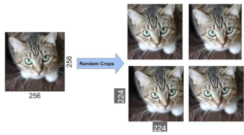 그림7. Data Augmentation
Code (tensorflow)
다음은 AlexNet을 텐서플로우를 사용한 코드로 확인해보겠습니다.
import numpy as np
import pandas as pd
import os
다음과 같이 기초적인 모듈들을 불러옵니다.
AlexNet 모델 생성
from tensorflow.keras.models import Model
from tensorflow.keras.layers import Input, Dense , Conv2D , Dropout , Flatten , Activation, MaxPooling2D , GlobalAveragePooling2D
from tensorflow.keras.optimizers import Adam , RMSprop
from tensorflow.keras.layers import BatchNormalization
from tensorflow.keras.callbacks import ReduceLROnPlateau , EarlyStopping , ModelCheckpoint , LearningRateScheduler
from tensorflow.keras import regularizers

# input shape, classes 개수, kernel_regularizer등을 인자로 가져감.
def create_alexnet(in_shape=(227, 227, 3), n_classes=10, kernel_regular=None):
    # 첫번째 CNN->ReLU->MaxPool, kernel_size를 매우 크게 가져감(11, 11)
    input_tensor = Input(shape=in_shape)

    x = Conv2D(filters= 96, kernel_size=(11,11), strides=(4,4), padding='valid')(input_tensor)
    x = Activation('relu')(x)
    # LRN을 대신하여 Batch Normalization 적용.
    x = BatchNormalization()(x)
    x = MaxPooling2D(pool_size=(3,3), strides=(2,2))(x)


    # 두번째 CNN->ReLU->MaxPool. kernel_size=(5, 5)
    x = Conv2D(filters=256, kernel_size=(5,5), strides=(1,1), padding='same',kernel_regularizer=kernel_regular)(x)
    x = Activation('relu')(x)
    x = BatchNormalization()(x)
    x = MaxPooling2D(pool_size=(3,3), strides=(2,2))(x)


    # 3x3 Conv 2번 연속 적용. filters는 384개
    x = Conv2D(filters=384, kernel_size=(3,3), strides=(1,1), padding='same', kernel_regularizer=kernel_regular)(x)
    x = Activation('relu')(x)
    x = BatchNormalization()(x)

    x = Conv2D(filters=384, kernel_size=(3,3), strides=(1,1), padding='same', kernel_regularizer=kernel_regular)(x)
    x = Activation('relu')(x)
    x = BatchNormalization()(x)

    # 3x3 Conv를 적용하되 filters 수를 줄이고 maxpooling을 적용
    x = Conv2D(filters=256, kernel_size=(3,3), strides=(1,1), padding='same', kernel_regularizer=kernel_regular)(x)
    x = Activation('relu')(x)
    x = BatchNormalization()(x)
    x = MaxPooling2D(pool_size=(3,3), strides=(2,2))(x)

    # Dense 연결을 위한 Flatten
    x = Flatten()(x)

    # Dense + Dropout을 연속 적용.
    x = Dense(units = 4096, activation = 'relu')(x)
    x = Dropout(0.5)(x)

    x = Dense(units = 4096, activation = 'relu')(x)
    x = Dropout(0.5)(x)

    # 마지막 softmax 층 적용.
    output = Dense(units = n_classes, activation = 'softmax')(x)

    model = Model(inputs=input_tensor, outputs=output)
    model.summary()

    return model
이렇게 위에서 설명한 AlexNet Architecture에 맞게끔 작성하였습니다.
CIFAR10 데이터세트를 이용하여 AlextNet 학습 및 성능 테스트
model = create_alexnet(in_shape=(227, 227, 3), n_classes=10, kernel_regular=regularizers.l2(l2=1e-4))
from tensorflow.keras.datasets import cifar10

# 전체 6만개 데이터 중, 5만개는 학습 데이터용, 1만개는 테스트 데이터용으로 분리
(train_images, train_labels), (test_images, test_labels) = cifar10.load_data()
print("train dataset shape:", train_images.shape, train_labels.shape)
print("test dataset shape:", test_images.shape, test_labels.shape)
학습/검증/테스트 데이터 세트로 나누고 데이터 전처리 수행
- 학습/검증/테스트 데이터로 분할. 검증 데이터는 학습 데이터의 20% 할당.
- 레이블의 원-핫 인코딩과 이미지 픽셀값의 스케일링 적용
import tensorflow as tf
import numpy as np
import pandas as pd

import random as python_random
from tensorflow.keras.utils import to_categorical
from sklearn.model_selection import train_test_split
from tensorflow.keras.datasets import cifar10

def zero_one_scaler(image):
    return image/255.0

def get_preprocessed_ohe(images, labels, pre_func=None):
    # preprocessing 함수가 입력되면 이를 이용하여 image array를 scaling 적용.
    if pre_func is not None:
        images = pre_func(images)
    # OHE 적용
    oh_labels = to_categorical(labels)
    return images, oh_labels

# 학습/검증/테스트 데이터 세트에 전처리 및 OHE 적용한 뒤 반환
def get_train_valid_test_set(train_images, train_labels, test_images, test_labels, valid_size=0.15, random_state=2021):
    # 학습 및 테스트 데이터 세트를  0 ~ 1사이값 float32로 변경 및 OHE 적용.
    train_images, train_oh_labels = get_preprocessed_ohe(train_images, train_labels)
    test_images, test_oh_labels = get_preprocessed_ohe(test_images, test_labels)

    # 학습 데이터를 검증 데이터 세트로 다시 분리
    tr_images, val_images, tr_oh_labels, val_oh_labels = train_test_split(train_images, train_oh_labels, test_size=valid_size, random_state=random_state)

    return (tr_images, tr_oh_labels), (val_images, val_oh_labels), (test_images, test_oh_labels )

# CIFAR10 데이터 재 로딩 및 Scaling/OHE 전처리 적용하여 학습/검증/데이터 세트 생성.
(train_images, train_labels), (test_images, test_labels) = cifar10.load_data()
print(train_images.shape, train_labels.shape, test_images.shape, test_labels.shape)
(tr_images, tr_oh_labels), (val_images, val_oh_labels), (test_images, test_oh_labels) = \
    get_train_valid_test_set(train_images, train_labels, test_images, test_labels, valid_size=0.2, random_state=2021)

print(tr_images.shape, tr_oh_labels.shape, val_images.shape, val_oh_labels.shape, test_images.shape, test_oh_labels.shape)


# 이미지 사이즈가 너무 작으면 모델의 MaxPooling에서 오류 발생.
model = create_alexnet(in_shape=(128, 128, 3), n_classes=10, kernel_regular=regularizers.l2(l2=1e-4))
CIFAR10 원본 이미지 크기 32x32 를 128x128로 증가 시키는 Sequence Dataset 생성
- 128x128로 CIFAR10 모든 이미지 배열값을 증가시키면 RAM 부족 발생.
- 배치 크기 만큼의 개수만 원본 이미지를 128x128로 증가 시킨 뒤(opencv의 resize()), 이를 모델에 입력하는 로직으로 Sequence Dataset 구성.
IMAGE_SIZE = 128
BATCH_SIZE = 64

from tensorflow.keras.utils import Sequence
import cv2
import sklearn

# 입력 인자 images_array labels는 모두 numpy array로 들어옴.
# 인자로 입력되는 images_array는 전체 32x32 image array임.
class CIFAR_Dataset(Sequence):
    def __init__(self, images_array, labels, batch_size=BATCH_SIZE, augmentor=None, shuffle=False, pre_func=None):
        '''
        파라미터 설명
        images_array: 원본 32x32 만큼의 image 배열값.
        labels: 해당 image의 label들
        batch_size: __getitem__(self, index) 호출 시 마다 가져올 데이터 batch 건수
        augmentor: albumentations 객체
        shuffle: 학습 데이터의 경우 epoch 종료시마다 데이터를 섞을지 여부
        '''
        # 객체 생성 인자로 들어온 값을 객체 내부 변수로 할당.
        # 인자로 입력되는 images_array는 전체 32x32 image array임.
        self.images_array = images_array
        self.labels = labels
        self.batch_size = batch_size
        self.augmentor = augmentor
        self.pre_func = pre_func
        # train data의 경우
        self.shuffle = shuffle
        if self.shuffle:
            # 객체 생성시에 한번 데이터를 섞음.
            #self.on_epoch_end()
            pass

    # Sequence를 상속받은 Dataset은 batch_size 단위로 입력된 데이터를 처리함.
    # __len__()은 전체 데이터 건수가 주어졌을 때 batch_size단위로 몇번 데이터를 반환하는지 나타남
    def __len__(self):
        # batch_size단위로 데이터를 몇번 가져와야하는지 계산하기 위해 전체 데이터 건수를 batch_size로 나누되, 정수로 정확히 나눠지지 않을 경우 1회를 더한다.
        return int(np.ceil(len(self.labels) / self.batch_size))

    # batch_size 단위로 image_array, label_array 데이터를 가져와서 변환한 뒤 다시 반환함
    # 인자로 몇번째 batch 인지를 나타내는 index를 입력하면 해당 순서에 해당하는 batch_size 만큼의 데이타를 가공하여 반환
    # batch_size 갯수만큼 변환된 image_array와 label_array 반환.
    def __getitem__(self, index):
        # index는 몇번째 batch인지를 나타냄.
        # batch_size만큼 순차적으로 데이터를 가져오려면 array에서 index*self.batch_size:(index+1)*self.batch_size 만큼의 연속 데이터를 가져오면 됨
        # 32x32 image array를 self.batch_size만큼 가져옴.
        images_fetch = self.images_array[index*self.batch_size:(index+1)*self.batch_size]
        if self.labels is not None:
            label_batch = self.labels[index*self.batch_size:(index+1)*self.batch_size]

        # 만일 객체 생성 인자로 albumentation으로 만든 augmentor가 주어진다면 아래와 같이 augmentor를 이용하여 image 변환
        # albumentations은 개별 image만 변환할 수 있으므로 batch_size만큼 할당된 image_name_batch를 한 건씩 iteration하면서 변환 수행.
        # 변환된 image 배열값을 담을 image_batch 선언. image_batch 배열은 float32 로 설정.
        image_batch = np.zeros((images_fetch.shape[0], IMAGE_SIZE, IMAGE_SIZE, 3), dtype='float32')

        # batch_size에 담긴 건수만큼 iteration 하면서 opencv image load -> image augmentation 변환(augmentor가 not None일 경우)-> image_batch에 담음.
        for image_index in range(images_fetch.shape[0]):
            #image = cv2.cvtColor(cv2.imread(image_name_batch[image_index]), cv2.COLOR_BGR2RGB)
            # 원본 image를 IMAGE_SIZE x IMAGE_SIZE 크기로 변환
            image = cv2.resize(images_fetch[image_index], (IMAGE_SIZE, IMAGE_SIZE))
            # 만약 augmentor가 주어졌다면 이를 적용.
            if self.augmentor is not None:
                image = self.augmentor(image=image)['image']

            # 만약 scaling 함수가 입력되었다면 이를 적용하여 scaling 수행.
            if self.pre_func is not None:
                image = self.pre_func(image)

            # image_batch에 순차적으로 변환된 image를 담음.
            image_batch[image_index] = image

        return image_batch, label_batch

    # epoch가 한번 수행이 완료 될 때마다 모델의 fit()에서 호출됨.
    def on_epoch_end(self):
        if(self.shuffle):
            #print('epoch end')
            # 원본 image배열과 label를 쌍을 맞춰서 섞어준다. scikt learn의 utils.shuffle에서 해당 기능 제공
            self.images_array, self.labels = sklearn.utils.shuffle(self.images_array, self.labels)
        else:
            pass

def zero_one_scaler(image):
    return image/255.0

tr_ds = CIFAR_Dataset(tr_images, tr_oh_labels, batch_size=BATCH_SIZE, augmentor=None, shuffle=True, pre_func=zero_one_scaler)
val_ds = CIFAR_Dataset(val_images, val_oh_labels, batch_size=BATCH_SIZE, augmentor=None, shuffle=False, pre_func=zero_one_scaler)

print(next(iter(tr_ds))[0].shape, next(iter(val_ds))[0].shape)
print(next(iter(tr_ds))[1].shape, next(iter(val_ds))[1].shape)
print(next(iter(tr_ds))[0][0])
Input 크기가 128x128x3 인 AlexNet 모델을 생성하고 epochs는 30으로 설정하고 학습
model = create_alexnet(in_shape=(128, 128, 3), n_classes=10, kernel_regular=regularizers.l2(l2=1e-4))

model.compile(optimizer=Adam(lr=0.001), loss='categorical_crossentropy', metrics=['accuracy'])

# 5번 iteration내에 validation loss가 향상되지 않으면 learning rate을 기존 learning rate * 0.2로 줄임.
rlr_cb = ReduceLROnPlateau(monitor='val_loss', factor=0.2, patience=5, mode='min', verbose=1)
ely_cb = EarlyStopping(monitor='val_loss', patience=10, mode='min', verbose=1)

history = model.fit(tr_ds, epochs=30,
                    #steps_per_epoch=int(np.ceil(tr_images.shape[0]/BATCH_SIZE)),
                    validation_data=val_ds,
                    #validation_steps=int(np.ceil(val_images.shape[0]/BATCH_SIZE)),
                    callbacks=[rlr_cb, ely_cb]
                   )

test_ds = CIFAR_Dataset(test_images, test_oh_labels, batch_size=BATCH_SIZE, augmentor=None, shuffle=False, pre_func=zero_one_scaler)
model.evaluate(test_ds)
이렇게 AlexNet의 이론적 설명을 논문을 통해서 알아보고 텐서플로우 코드로 작성해보았습니다. 봐주셔서 감사합니다😀😀
출저
[1] https://deep-learning-study.tistory.com/376
[2] https://bskyvision.com/421
[3] https://m.blog.naver.com/laonple/220654387455
