Summary

Fast R-CNN revolutionizes object detection by addressing the key limitations of R-CNN. It introduces RoI Pooling, enabling more efficient computation and better utilization of shared feature maps, but it still primarily relies on CPUs, limiting its speed.

---

Introduction

Limitations of R-CNN

R-CNN brought significant advancements to object detection but still suffered from several key challenges.
1. Slow Training: Training R-CNN on large datasets like the PASCAL VOC dataset takes about 84 hours and consumes considerable disk space.
2. Slow Inference: Detection takes 47 seconds per image with VGG16.
3. Spatial Distortion: Warping region proposals to a fixed size (227x227) introduces spatial loss.
4. Inefficient Region Proposal Processing: Each of the 2000 region proposals is processed independently through the CNN, leading to redundant computations and slow performance.

Fast R-CNN addresses these issues by rethinking how region proposals and features are processed, making detection faster and more efficient. R-CNN's inefficiencies paved the way for Fast R-CNN, which optimizes object detection with a unified and efficient pipeline, significantly improving speed and accuracy.

Let's dig in.

---

Object Detection with Fast R-CNN

Model Overview:

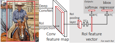
Fast R-CNN Workflow

• 1. The input image is passed through a CNN backbone to generate a feature map.
• 2. Region proposals are extracted using Selective Search to identify potential object regions.
• 3. The region proposals are projected onto the shared feature map to align them with the convolutional features.
• 4. RoI Pooling is applied to convert each region proposal into a fixed-sized feature map.
• 5. Fully Connected Layers (FCLs) perform classification and bounding-box regression, optimized with a multi-task loss.

Detailed Architecture of Fast R-CNN

Spatial Pyramid Pooling (SPP)

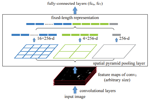
• Fast R-CNN builds on the idea of Spatial Pyramid Pooling (SPP) from SPPnet. While SPP divides the feature map into multiple levels to create fixed-size feature vectors, capturing multi-scale spatial information.

• Fast R-CNN simplifies this by using RoI Pooling, which directly converts each RoI into a fixed-size 7x7 feature map. This approach retains the benefits of SPP while significantly reducing computational complexity.

• Instead of resizing input images to a fixed size, Fast R-CNN processes the entire image through a CNN to generate a shared convolutional feature map, which is then used by RoI Pooling to handle region proposals of varying sizes.

The RoI pooling layer

RoI Pooling is a key component in Fast R-CNN that converts region proposals into fixed-size feature maps. Dividing the feature map of a RoI into a fixed grid and applying max pooling to each cell standardizes the output size, enabling consistent processing in FCLs.

Step 1) Feature Map Extraction via CNN Backbone

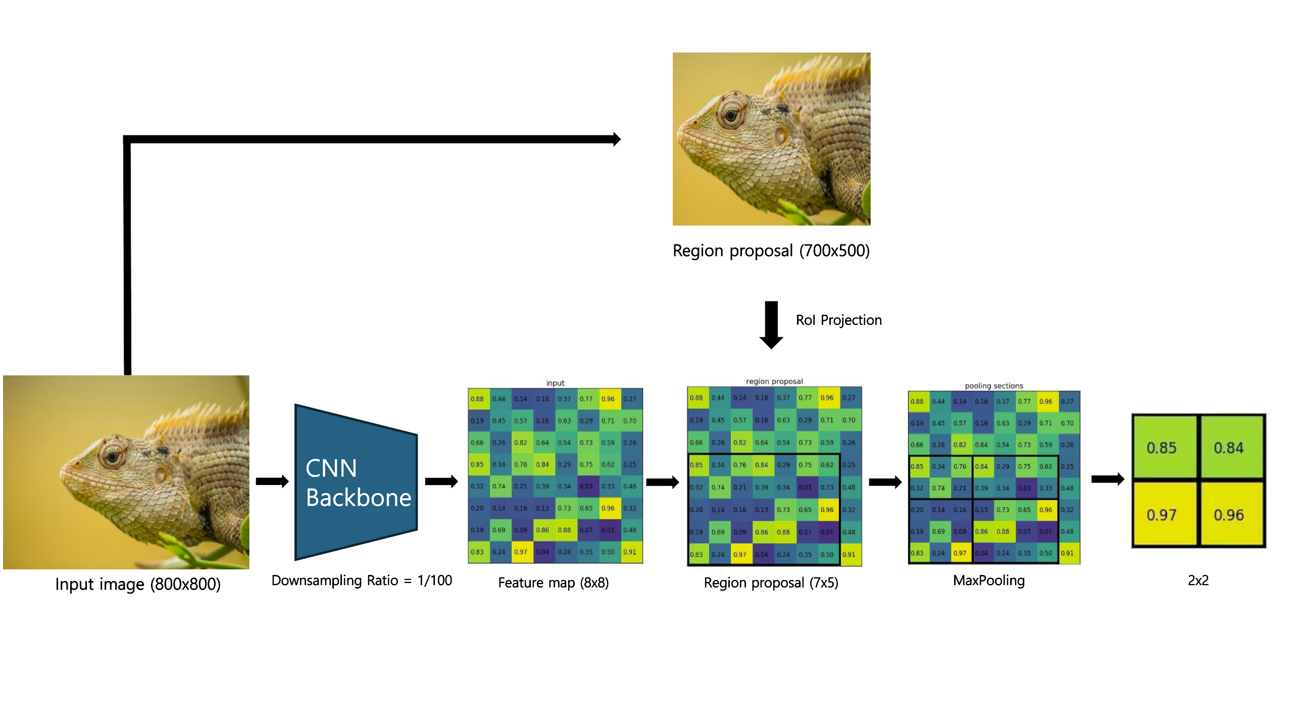
• The input image is passed through a CNN backbone (e.g., VGG16) to extract a feature map.
• The feature map has a reduced spatial resolution compared to the original image, determined by the downsampling ratio of the CNN.
  • For example: An 800 x 800 input image generates a feature map of size 8 x 8 with a downsampling ratio of 1/100.
  • Each pixel on the feature map corresponds to a 100 x 100 region in the original image.

Step 2) Region Proposal Generation

• Selective Search Algorithm identifies the Region of Interest (RoI) in the input image.
• Each RoI is represented by:
  • A four-tuple (r, c, h, w) where:
    • r, c: Top-left corner coordinates
    • h, w: Height and width of the region
• These proposals mark the areas most likely to contain objects for further analysis.

Step 3) RoI Projection

• The coordinates of each RoI, defined in the original image space, are projected onto the feature map. This involves scaling the RoI dimensions using the downsampling ratio of the CNN.
  • For Example: An RoI with dimensions (700, 500) in the original image maps to a 7 x 5 region on the 8 x 8 feature map.

Step 4) Grid Division

• The projected RoI on the feature map is divided into a fixed grid of size H x W.
• Each grid cell corresponds to a sub-region of the RoI. The size of each grid cell is approximately:
  • Grid cell size = h/H x w/W

Step 5) Max Pooling

• Max pooling is applied independently to each grid cell, and the maximum value is selected to represent that cell.
• This step generates a fixed-size feature map for each RoI, preserving key spatial features while standardizing the dimensions.

Output: Fixed-size Feature Map
- The fixed-size feature maps produced by RoI Pooling are flattened into feature vectors and passed through FCLs for:
- Classification: Softmax over K + 1 categories
- Bounding-Box Regression: Category-specific bounding-box regressor

Hierarchical sampling

• SPPnet's Limitations:
  • SPPnet struggles with backpropagation due to the large receptive fields of RoIs, often spanning the entire image.
  • Each RoI requires processing the entire receptive field of the original image, making backpropagation computationally expensive.
• Fast R-CNN's Solution:
  • Hierarchical mini-batch sampling
    • First, N images are sampled, followed by R/N RoIs per image.
    • Example: With N = 2 and R = 128, this method is 64x faster than R-CNN's method of sampling one RoI from 128 different images.
• Streamlined Training Process:
  Fast R-CNN optimizes both classification and bounding-box regression in a single fine-tuning stage, replacing R-CNN's stage-wise approach:
  • R-CNN: Trains a softmax classifier, SVMs, and regressor separately.
  • Fast R-CNN: Jointly optimizes a softmax classifier and bounding-box regressors.

Multi-task Loss

A Fast R-CNN network has two sibling output layers, designed to jointly handle classification and bounding-box regression. This multi-task loss framework ensures that both tasks are optimized simultaneously, providing efficient and accurate object detection.

1. Classification Loss:

• Outputs a discrete probability distribution per RoI over K + 1 categories (including the background class).
• Defined as:
  

2. Bounding-box Regression Loss:
   Refines bounding-box predictions for object localization.
   Applies only to non-background classes (𝑢≥1).
   Defined as:
   

t: Predicted bounding-box offsets
v: Ground-truth bounding-box targets

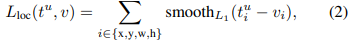
Combined Loss Function
The overall multi-task loss is defined as:
λ: Balancing factor for the two loss terms (commonly λ = 1)
[𝑢≥1]: Ensures that bounding-box regression is only applied to non-background RoIs. (u = 0, if it's background)

Truncated SVD for faster detection

For detection, the processing of a large number of RoIs significantly increases computational demands, with nearly half of the forward pass time spent on the fully connected layers.
To address this bottleneck, Fast R-CNN leverages Truncated Singular Value Decomposition (SVD) to compress these large fully connected layers, accelerating computations and reducing processing time effectively.

How Truncated SVD Works

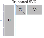
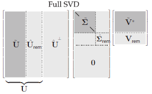
• 1. Matrix Factorization:
  The weight matrix W (u x v) in the FCL is factorized into three smaller matrices:
  

U: A 𝑢×𝑡 matrix containing the first 𝑡 left singular vectors.
Σₜ: A t×t diagonal matrix with the top t singular values.
V: A v×t matrix containing the first t right singular vectors.

• 2. Compression:

  • The original parameter count uv is reduced to t(u+v), where t≪min(u,v).

  • This compression significantly decreases the number of computations required in the fully connected layers, resulting in faster forward passes.

3. Layer Substitution:
The fully connected layer using W is replaced by two smaller layers:
First Layer: Uses Σₜ Vᵀ as weights.
Second Layer: Uses U as weights, along with the original biases.

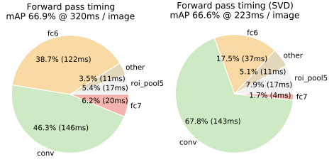
Truncated SVD can reduce detection time by more than 30%, achieving significant computational efficiency with minimal impact on detection accuracy.

---

Performance

Fast R-CNN exhibits remarkable improvements in both accuracy and speed over R-CNN:

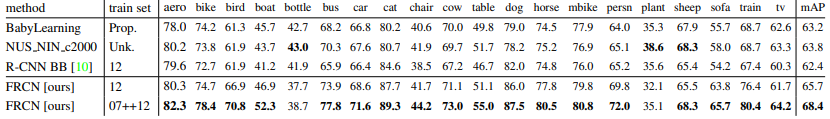
• Mean Average Precision (mAP):

  • Achieved 68.4% on the PASCAL VOC 2012 dataset, showcasing robust detection accuracy.

• Speed Enhancement:

  • 146× Faster than R-CNN without Truncated SVD.
  • 213× Faster with Truncated SVD, resulting in an additional 30% reduction in detection time.

• Revolutionary Improvements:

  • Introduced RoI Pooling, enabling efficient processing of region proposals by reusing shared convolutional feature maps.
  • Balanced speed and accuracy for large-scale object detection tasks.
    

Fast R-CNN revolutionized object detection by addressing R-CNN's inefficiencies, significantly enhancing both training and inference speeds while maintaining strong detection accuracy.

---

Conclusion

Fast R-CNN marks a pivotal advancement in object detection by addressing the key limitations of its predecessor, R-CNN, while introducing innovative features like RoI Pooling and a one-stage training structure. Here's how Fast R-CNN overcomes the challenges faced by R-CNN:

---

R-CNN's Limitations and Fast R-CNN's Solutions

R-CNN Limitation	Fast R-CNN Solution
Slow Training: Training on large datasets takes over 84 hours and consumes significant disk space.	Jointly optimizes classification and bounding-box regression in a single stage, drastically reducing training time.
Slow Inference: Detection takes 47 seconds per image with VGG16.	Shared computation of feature maps and RoI Pooling significantly reduce inference time (up to 213x faster).
Spatial Distortion: Warping region proposals to fixed size (227x227) causes spatial loss.	RoI Pooling extracts fixed-size features without distorting the input regions, preserving spatial information.
Inefficient Region Proposal Processing: Each of the 2,000 proposals is processed independently through the CNN, leading to redundancy.	Processes the entire image once through the CNN backbone to generate shared feature maps, avoiding redundant computations.

---

Fast R-CNN's Limitations

While Fast R-CNN resolves many of R-CNN's inefficiencies, it introduces its own challenges:

1. Region Proposal Bottleneck:

   • Fast R-CNN still relies on external algorithms like Selective Search for generating region proposals, which are computationally expensive and predominantly CPU-based. This bottleneck limits its potential for real-time applications.

2. GPU Utilization:

   • Unlike later models such as Faster R-CNN, which integrates region proposal generation within the network, Fast R-CNN cannot fully leverage the computational power of GPUs for an end-to-end pipeline.

---

Reflection

The most fascinating aspect of Fast R-CNN lies in how a seemingly simple change—introducing RoI Pooling to produce fixed-size feature maps at the right stage—leads to such a profound impact on performance. This adjustment, though small in concept, revolutionized object detection by enabling faster and more efficient computation, showcasing how minor innovations in architectural design can yield transformative results. It’s a reminder of the elegance and power of optimizing processes at the right place.

---

References

Girshick, R. (2015). Fast R-CNN. 2015 IEEE International Conference on Computer Vision (ICCV).
https://doi.org/10.1109/iccv.2015.169

He, K., Zhang, X., Ren, S., & Sun, J. (2015). Spatial pyramid pooling in deep convolutional networks for visual recognition. IEEE Transactions on Pattern Analysis and Machine Intelligence, 37(9), 1904–1916.
https://doi.org/10.1109/tpami.2015.2389824

Singular value decomposition (SVD). (2019). Data-Driven Science and Engineering, 3–46. https://doi.org/10.1017/9781108380690.002

Li, F.-F., Jonhson, J., & Yeung, S. (2017). Lecture 11: Detection and segmentation. https://cs231n.stanford.edu/slides/2017/cs231n_2017_lecture11.pdf

Grel, T. (2017, March 15). Region of interest pooling explained. deepsense.ai. Retrieved from https://deepsense.ai/region-of-interest-pooling-explained