폐렴 진단기 성능개선하기
- 캐글의 Chest X-Ray Images 사용
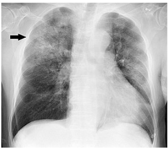
- 폐렴은 폐에 염증이 생긴 상태로 중증의 호흡기 감염병입니다.
폐렴 구별법
아래 이미지처럼 폐부위에 희미한 그림자?같은게 보이는데 사실 이 사진만으로 확실히 폐렴이다 아니다 판단하기 어렵습니다. 그래서 CNN모델을 이용해 구분을 해주는 모델을 만들어 보겠습니다.
Step 1. 실험환경 Set-up
import os, re
import random, math
import numpy as np
import tensorflow as tf
import matplotlib.pyplot as plt- 이미지 사이즈는 (180,180) 크기로 했지만 사이즈를 바꿔가면서 모델에 적용하는 것도 정답도를 올리는 하나의 방법일 것 같습니다.
- Batch Size는 몇으로 하는지에 따라 정확도에 변화가 있습니다. Epochs는 earlystopping을 이용할 것이기 때문에 충분히 크게 하면 될 것 같습니다.
# 데이터 로드할 때 빠르게 로드할 수 있도록하는 설정 변수
AUTOTUNE = tf.data.experimental.AUTOTUNE
# X-RAY 이미지 사이즈 변수
IMAGE_SIZE = [180, 180]

# 데이터 경로 변수
ROOT_PATH = os.path.join(os.getenv('HOME'), 'aiffel')
TRAIN_PATH = ROOT_PATH + '/chest_xray/data/train/*/*'
VAL_PATH = ROOT_PATH + '/chest_xray/data/val/*/*'
TEST_PATH = ROOT_PATH + '/chest_xray/data/test/*/*'
# 프로젝트를 진행할 때 아래 두 변수를 변경해보세요
BATCH_SIZE = 30
EPOCHS = 50
print(ROOT_PATH)Step 2. 데이터 준비하기
데이터에는
- train 5216
- test 624
- val 16
train_filenames = tf.io.gfile.glob(TRAIN_PATH)
test_filenames = tf.io.gfile.glob(TEST_PATH)
val_filenames = tf.io.gfile.glob(VAL_PATH)

print(len(train_filenames))
print(len(test_filenames))
print(len(val_filenames))
5216
624
16
val데이터가 16개로 적기 때문에 train에서 val으로 사용할 데이터 셋을 8:2분리를 하겠습니다.
# train 데이터와 validation 데이터를 모두 filenames에 담습니다
filenames = tf.io.gfile.glob(TRAIN_PATH)
filenames.extend(tf.io.gfile.glob(VAL_PATH))

# 모아진 filenames를 8:2로 나눕니다
train_size = math.floor(len(filenames)*0.8)
random.shuffle(filenames)
train_filenames = filenames[:train_size]
val_filenames = filenames[train_size:]

print(len(train_filenames))
print(len(val_filenames))
4185
1047
train 이미지중에서 폐렴인 이미지는 3097개 이고 아닌 이미지는 1088의 이미지 입니다.
# 정상 이미지와 폐렴 이미지를 구분해야 하는데
# 다행히도 파일 경로에 힌트가 있어요
print(f'Normal image path\n{filenames[0]}')
print(f'Pneumonia image path\n{filenames[2000]}')
Normal image path
/aiffel/aiffel/chest_xray/data/train/NORMAL/IM-0717-0001.jpeg
Pneumonia image path
/aiffel/aiffel/chest_xray/data/train/PNEUMONIA/person803_bacteria_2710.jpeg
# 이제 파일 경로에 NORMAL이 있는지 확인하면 정상 이미지를 셀 수 있습니다.
COUNT_NORMAL = len([filename for filename in train_filenames if "NORMAL" in filename])
print(f"Normal images count in training set: {COUNT_NORMAL}")

# 파일 경로에 PNEUMONIA이 있는지 확인하면 폐렴 이미지도 셀 수 있습니다.
COUNT_PNEUMONIA = len([filename for filename in train_filenames if "PNEUMONIA" in filename])
print(f"Pneumonia images count in training set: {COUNT_PNEUMONIA}")
Normal images count in training set: 1081
Pneumonia images count in training set: 3104
tf.data.Dataset.from_tensor_slices 함수는 tf.data.Dataset 를 생성하는 함수로 입력된 텐서로부터 slices를 생성합니다
train_list_ds = tf.data.Dataset.from_tensor_slices(train_filenames)
val_list_ds = tf.data.Dataset.from_tensor_slices(val_filenames)
tf.data에 잘 들어갔는지 확인합니다
TRAIN_IMG_COUNT = tf.data.experimental.cardinality(train_list_ds).numpy()
print(f"Training images count: {TRAIN_IMG_COUNT}")

VAL_IMG_COUNT = tf.data.experimental.cardinality(val_list_ds).numpy()
print(f"Validating images count: {VAL_IMG_COUNT}")
Training images count: 4185
Validating images count: 1047
파일 경로에 'NORMAL'이나 'PNEUMONIA'가 포함되어 있기 때문에 이를 이용해서 라벨 데이터를 만들어 주는 함수를 만들어 보겠습니다.
# 파일 경로의 끝에서 두번째 부분을 확인하면 양성과 음성을 구분할 수 있습니다
def get_label(file_path):
    parts = tf.strings.split(file_path, os.path.sep)
    return parts[-2] == "PNEUMONIA"   # 폐렴이면 양성(True), 노말이면 음성(False)
이미지의 사이즈를 통일 시키고 GPU 메모리를 더욱 효율적으로 사용하기 위해 이미지 사이즈를 줄여봅시다.
# 이미지를 알맞은 형식으로 바꿉니다.
def decode_img(img):
    img = tf.image.decode_jpeg(img, channels=3) # 이미지를 uint8 tensor로 수정
    img = tf.image.convert_image_dtype(img, tf.float32) # float32 타입으로 수정
    img = tf.image.resize(img, IMAGE_SIZE) # 이미지 사이즈를 IMAGE_SIZE로 수정
    return img

# 이미지 파일의 경로를 입력하면 이미지와 라벨을 읽어옵니다.
def process_path(file_path):
    label = get_label(file_path) # 라벨 검출
    img = tf.io.read_file(file_path) # 이미지 읽기
    img = decode_img(img) # 이미지를 알맞은 형식으로 수정
    return img, label
train 데이터 셋과 validation 데이터 셋을 만듭니다.
- num_parallel_calls 파라미터에서 set-up에서 초기화한 AUTOTUNE을 이용하면 빠르게 데이터를 처리해준다고 하네요?
train_ds = train_list_ds.map(process_path, num_parallel_calls=AUTOTUNE)
val_ds = val_list_ds.map(process_path, num_parallel_calls=AUTOTUNE)
이미지가 잘 들어갔는지 확인해보겠습니다.
for image, label in train_ds.take(1):
    print("Image shape: ", image.numpy().shape)
    print("Label: ", label.numpy())
Image shape: (180, 180, 3)
Label: False
위 작업은 train과 val만 했다면 test도 동일한 작업을 해줍니다!
test_list_ds = tf.data.Dataset.list_files(TEST_PATH)
TEST_IMAGE_COUNT = tf.data.experimental.cardinality(test_list_ds).numpy()
test_ds = test_list_ds.map(process_path, num_parallel_calls=AUTOTUNE)
test_ds = test_ds.batch(BATCH_SIZE)

print(TEST_IMAGE_COUNT)
624
위에서 Tensorflow에 data로 형성하고 효육적으로 사용하게 했습니다.
- random_flip_left_right 함수를 이용해 좌우 반전을 이용합니다.
- 함수를 형성하여 학습 데이터를 효육적으로 작동하도록 데이터를 변환합니다.
- shuffle은 고정 크기 버퍼를 유지하고 뮤작위로 균일하게 다음 요소를 선택합니다.
- repeat은 여러 번 데이터를 불러오게 합니다.
- batch는 정한 만큼의 배치로 주어집니다.
- prefech는 GPU와 CPU를 효율적으로 사용하는데 도움을 줍니다.
def augment(image,label):
    image = tf.image.random_flip_left_right(image)  # 랜덤하게 좌우를 반전합니다.
    return image,label

def prepare_for_training(ds, shuffle_buffer_size=1000):
    # augment 적용 부분이 배치처리 함수에 추가되었습니다.
    ds = ds.map(
            augment,       # augment 함수 적용
            num_parallel_calls=2
        )
    ds = ds.shuffle(buffer_size=shuffle_buffer_size)
    ds = ds.repeat()
    ds = ds.batch(BATCH_SIZE)
    ds = ds.prefetch(buffer_size=AUTOTUNE)

    return ds

train_ds = prepare_for_training(train_ds)
val_ds = prepare_for_training(val_ds)
Step 3. 데이터 시각화
데이터를 보기 위해 먼저, train에 있는 batch 중 첫 번째 배치를 추출합니다. 추출된 배치를 image와 label 데이터 셋으로 나눕니다.
# 이미지 배치를 입력하면 여러장의 이미지를 보여줍니다.
def show_batch(image_batch, label_batch):
    plt.figure(figsize=(10,10))
    for n in range(BATCH_SIZE):
        ax = plt.subplot(5,math.ceil(BATCH_SIZE/5),n+1)
        plt.imshow(image_batch[n])
        if label_batch[n]:
            plt.title("PNEUMONIA")
        else:
            plt.title("NORMAL")
        plt.axis("off")


image_batch, label_batch = next(iter(train_ds))
show_batch(image_batch.numpy(), label_batch.numpy())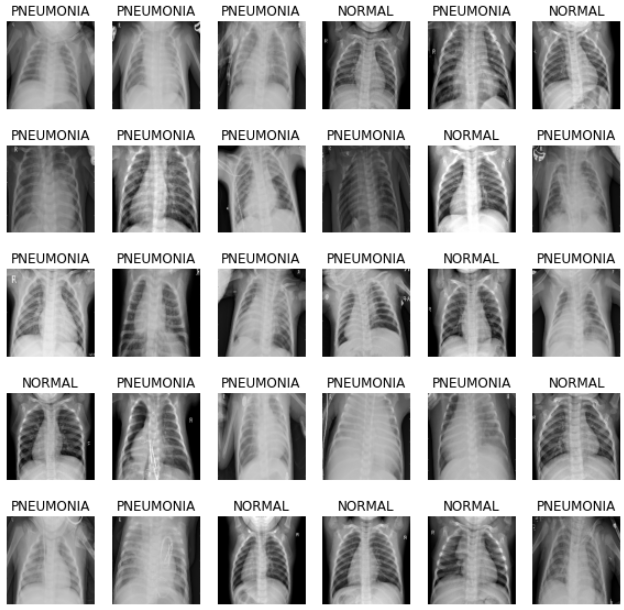
Step 4. CNN 모델링
- convolution block을 만듭니다.
- conv를 두번 시행
- batch Nomal을 통한 과적합 방지
- max pooling
def conv_block(filters):
    block = tf.keras.Sequential([
        tf.keras.layers.SeparableConv2D(filters, 3, activation='relu', padding='same'),
        tf.keras.layers.SeparableConv2D(filters, 3, activation='relu', padding='same'),
        tf.keras.layers.BatchNormalization(),
        tf.keras.layers.MaxPool2D()
    ])

return block- dense block
def dense_block(units, dropout_rate):
    block = tf.keras.Sequential([
        tf.keras.layers.Dense(units, activation='relu'),
        tf.keras.layers.BatchNormalization(),
        tf.keras.layers.Dropout(dropout_rate)
    ])

return block- 전체 모델 구축
def build_model():
    model = tf.keras.Sequential([
        tf.keras.Input(shape=(IMAGE_SIZE[0], IMAGE_SIZE[1], 3)),

        tf.keras.layers.Conv2D(16, 3, activation='relu', padding='same'),
        tf.keras.layers.Conv2D(16, 3, activation='relu', padding='same'),
        tf.keras.layers.MaxPool2D(),

        conv_block(32),
        conv_block(64),

        conv_block(128),
        tf.keras.layers.Dropout(0.2),

        conv_block(256),
        tf.keras.layers.Dropout(0.2),

        tf.keras.layers.Flatten(),
        dense_block(512, 0.7),
        dense_block(128, 0.5),
        dense_block(64, 0.3),

        tf.keras.layers.Dense(1, activation='sigmoid')
    ])

    return model
Step 5. 데이터 imbalance 처리
아까 데이터의 라벨양을 보면 폐렴의 이미지가 너무 많습니다. 그래서 각 라벨에 가중치를 주어 언벨런스한 부분을 어느정도 해결하겠습니다.
weight_for_0 = (1 / COUNT_NORMAL)*(TRAIN_IMG_COUNT)/2.0
weight_for_1 = (1 / COUNT_PNEUMONIA)*(TRAIN_IMG_COUNT)/2.0

class_weight = {0: weight_for_0, 1: weight_for_1}

print('Weight for NORMAL: {:.2f}'.format(weight_for_0))
print('Weight for PNEUMONIA: {:.2f}'.format(weight_for_1))
Weight for NORMAL: 1.94
Weight for PNEUMONIA: 0.67
Step 6. 모델 훈련
with tf.device('/GPU:0'):
    model = build_model()

    METRICS = [
        'accuracy',
        tf.keras.metrics.Precision(name='precision'),
        tf.keras.metrics.Recall(name='recall')
    ]

    model.compile(
        optimizer='adam',
        loss='binary_crossentropy',
        metrics=METRICS
    )
from keras.callbacks import EarlyStopping
# 최고의 정확도를 가질때 멈춰주는 함수 추가
es=EarlyStopping(monitor='val_loss',mode='min',verbose=1,patience=10)with tf.device('/GPU:0'):
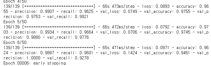
history = model.fit(
train_ds,
steps_per_epoch=TRAIN_IMG_COUNT // BATCH_SIZE,
epochs=EPOCHS,callbacks=[es],
validation_data=val_ds,
validation_steps=VAL_IMG_COUNT // BATCH_SIZE,
class_weight=class_weight,
)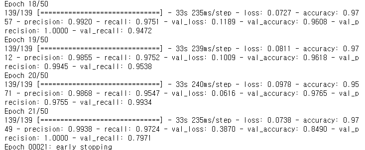
Step 7. 결과 확인과 시각화
위 모델 결과를 바탕으로 그래프로 Epochs마다 모델의 precision, recall, accuracy, loss의 변화를 보겠습니다.
fig, ax = plt.subplots(1, 4, figsize=(20, 3))
ax = ax.ravel()

for i, met in enumerate(['precision', 'recall', 'accuracy', 'loss']):
    ax[i].plot(history.history[met])
    ax[i].plot(history.history['val_' + met])
    ax[i].set_title('Model {}'.format(met))
    ax[i].set_xlabel('epochs')
    ax[i].set_ylabel(met)
    ax[i].legend(['train', 'val'])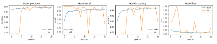
test데이터로 모델을 평가해봅니다.
loss, accuracy, precision, recall = model.evaluate(test_ds)
print(f'Loss: {loss},\nAccuracy: {accuracy},\nPrecision: {precision},\nRecall: {recall}')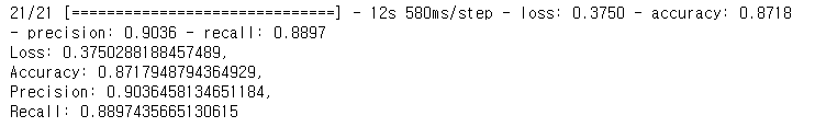
위 결과는 recall값이 매우 작네요! 의료데이터는 실제 폐렴인 환자를 정상으로 판단하면 매우 위험하기 때문에 recall값을 올려야합니다. recall값이 높아 질 수 있도록 다시 학습을 해보겠습니다.
Recall값을 올리자
위에서 의료데이터를 좌우반전도 해서 학습시키는 작업을 했습니다. 하지만 X ray사진을 찍을때 항상 같은 조건으로 촬영을 합니다. 그래서 좌우반전 작업을 삭제하고 다시해보겠습니다.
test_list_ds = tf.data.Dataset.list_files(TEST_PATH)
TEST_IMAGE_COUNT = tf.data.experimental.cardinality(test_list_ds).numpy()
test_ds = test_list_ds.map(process_path, num_parallel_calls=AUTOTUNE)
test_ds = test_ds.batch(BATCH_SIZE)
좌우반전 함수 삭제
def prepare_for_training(ds, shuffle_buffer_size=1000):
    ds = ds.shuffle(buffer_size=shuffle_buffer_size)
    ds = ds.repeat()
    ds = ds.batch(BATCH_SIZE)
    ds = ds.prefetch(buffer_size=AUTOTUNE)
    return ds

train_ds = prepare_for_training(train_ds)
val_ds = prepare_for_training(val_ds)
conv2D레이어 256 --> 128 -->64-->128-->256 등의 형태로 변경
def build_model():
    model = tf.keras.Sequential([
        tf.keras.Input(shape=(IMAGE_SIZE[0], IMAGE_SIZE[1], 3)),

        tf.keras.layers.Conv2D(128, 3, activation='relu', padding='same'),
        tf.keras.layers.Conv2D(64, 3, activation='relu', padding='same'),
        tf.keras.layers.MaxPool2D(),

        conv_block(64),
        conv_block(64),

        conv_block(128),
        tf.keras.layers.Dropout(0.2),

        conv_block(256),
        tf.keras.layers.Dropout(0.2),

        tf.keras.layers.Flatten(),
        dense_block(512, 0.7),
        dense_block(128, 0.5),
        dense_block(64, 0.3),

        tf.keras.layers.Dense(1, activation='sigmoid')
    ])

    return model
with tf.device('/GPU:0'):
    model = build_model()

    METRICS = [
        'accuracy',
        tf.keras.metrics.Precision(name='precision'),
        tf.keras.metrics.Recall(name='recall')
    ]

    model.compile(
        optimizer='adam',
        loss='binary_crossentropy',
        metrics=METRICS
    )
BATCH_SIZE 50 -->16으로 변경
BATCH_SIZE = 30
EPOCHS = 50
earlystopping은 val precision을 기준으로 멈추겠습니다!
- 왜 recall이 아니라 precision이냐구여? recall이 높은 게 좋긴한데 recall을 기준으로 하면 precision이나 accuracy가 매우 낮게 나오더라구여... ㅠㅠ 그래서 presicion으로 해보니까 골고루? 좋게나와서 presicion기준으로 했습니다.
from keras.callbacks import EarlyStopping
# 최고의 정확도를 가질때 멈춰주는 함수 추가
es=EarlyStopping(monitor='val_precision',mode='max',verbose=1,patience=5)
with tf.device('/GPU:0'):
history = model.fit(
train_ds,
steps_per_epoch=TRAIN_IMG_COUNT // BATCH_SIZE,
epochs=EPOCHS,callbacks=[es],
validation_data=val_ds,
validation_steps=VAL_IMG_COUNT // BATCH_SIZE,
class_weight=class_weight,
)
loss, accuracy, precision, recall = model.evaluate(test_ds)
print(f'Loss: {loss},\nAccuracy: {accuracy},\nPrecision: {precision},\nRecall: {recall}')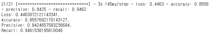
아까 위의 21에폭이나 하고 Recall: 0.8897435665130615 보다는 약간 변형을 준 바로 위 모델이 recall값이 더 좋은 결과를 가지고 왔습니다. 사실 recall을 99까지 올릴수 있지만 그렇게 하면 다른 precision이나 accuracy값이 매우 낮아서... 약간 포기해봤습니다.
마지막은 세개 모두 올리는 방향으로 해보겠습니다!
BATCH_SIZE = 16
EPOCHS = 80
from keras.callbacks import EarlyStopping
# 최고의 정확도를 가질때 멈춰주는 함수 추가
es=EarlyStopping(monitor='val_loss',mode='min',verbose=1,patience=20)with tf.device('/GPU:0'):
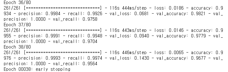
history = model.fit(
train_ds,
steps_per_epoch=TRAIN_IMG_COUNT // BATCH_SIZE,
epochs=EPOCHS,callbacks=[es],
validation_data=val_ds,
validation_steps=VAL_IMG_COUNT // BATCH_SIZE,
class_weight=class_weight,
)
loss, accuracy, precision, recall = model.evaluate(test_ds)
print(f'Loss: {loss},\nAccuracy: {accuracy},\nPrecision: {precision},\nRecall: {recall}')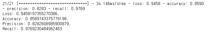
early stop을 val_loss로 설정하는게 고루고루 좋은 값을 보이는 것 같습니다. 의료데이터는 recall값을 중요시 하기때문에 다른건 무시하고 recall값을 100%에 가깝게 하겠다! 하면 early stop을 recall로 설정해서 모델을 구축하는게 더 좋은 모델일 수도 있겠네요!! 인공지능 특성상 100% 정확도를 가지는 모델을 만들기 힘들다보니 하나를 얻으려면 다른것을 잃어야하는건 어쩔수없나봅니다 ㅜㅜ 튼 그렇습니다! 여러 하이퍼파라미터를 바꿔보면서 해본 실험이였습니다.!