
📌 사용 환경
Python 3.10.2
conda 24.9.0
JupyterLab 4.2.5
판다스에서 데이터 셋을 제공하는 것처럼 사이킷런에서도 제공한다.
그중 소규모의 연습용 데이터 셋인 붓꽃 데이터셋을 가져올 것이다.
1. 붓꽃 품종 데이터셋
https://scikit-learn.org/stable/modules/generated/sklearn.datasets.load_iris.html#load-iris
사용할 라이브러리를 먼저 import해주고,
import numpy as np
import pandas as pd
import seaborn as sns

import matplotlib.pyplot as plt
import matplotlib as mpl
mpl.rc("font", family="Malgun Gothic")
plt.rcParams["axes.unicode_minus"]=False

from sklearn.neighbors import KNeighborsClassifier
from sklearn.model_selection import train_test_split
from sklearn.preprocessing import StandardScaler, MinMaxScaler, RobustScaler
from sklearn.preprocessing import LabelEncoder, OneHotEncoder
이번에는 sckitlearn에서 제공하는 데이터셋인 붓꽃 품종 데이터를 또 import해줘야한다.
from sklearn.datasets import load_iris이제 데이터를 가져오자.
iris=load_iris()
type(iris)sklearn.utils._bunch.Bunch여기서 이 bunch라는 것은 사이킷런에서 만든 것이다.
이는 딕셔너리와 유사하며 keys()를 찍어보면 다음과 같다.
iris.keys()dict_keys(['data', 'target', 'frame', 'target_names', 'DESCR', 'feature_names', 'filename', 'data_module'])여기서 X가 data, X의 이름이 feature_name, Y가 target, Y의 이름이 target_names다.
이제 각각의 데이터의 타입을 또 확인해야한다.
print(type(iris.data), type(iris.feature_names))  # 설명변수 X
print(type(iris.target), type(iris.target_names)) # 목표변수 Y<class 'numpy.ndarray'> <class 'list'>
<class 'numpy.ndarray'> <class 'numpy.ndarray'>그리고 DESCR은 데이터를 설명해주는 문자열이다.
print(iris.DESCR).. _iris_dataset:
Iris plants dataset
--------------------
**Data Set Characteristics:**
:Number of Instances: 150 (50 in each of three classes)
:Number of Attributes: 4 numeric, predictive attributes and the class
:Attribute Information:
- sepal length in cm
- sepal width in cm
- petal length in cm
- petal width in cm
- class:
- Iris-Setosa
- Iris-Versicolour
- Iris-Virginica
:Summary Statistics:
============== ==== ==== ======= ===== ====================
Min Max Mean SD Class Correlation
============== ==== ==== ======= ===== ====================
sepal length: 4.3 7.9 5.84 0.83 0.7826
sepal width: 2.0 4.4 3.05 0.43 -0.4194
petal length: 1.0 6.9 3.76 1.76 0.9490 (high!)
petal width: 0.1 2.5 1.20 0.76 0.9565 (high!)
============== ==== ==== ======= ===== ====================
:Missing Attribute Values: None
:Class Distribution: 33.3% for each of 3 classes.
:Creator: R.A. Fisher
:Donor: Michael Marshall (MARSHALL%PLU@io.arc.nasa.gov)
:Date: July, 1988
The famous Iris database, first used by Sir R.A. Fisher. The dataset is taken
from Fisher's paper. Note that it's the same as in R, but not as in the UCI
Machine Learning Repository, which has two wrong data points.
This is perhaps the best known database to be found in the
pattern recognition literature. Fisher's paper is a classic in the field and
is referenced frequently to this day. (See Duda & Hart, for example.) The
data set contains 3 classes of 50 instances each, where each class refers to a
type of iris plant. One class is linearly separable from the other 2; the
latter are NOT linearly separable from each other.
.. topic:: References
- Fisher, R.A. "The use of multiple measurements in taxonomic problems"
Annual Eugenics, 7, Part II, 179-188 (1936); also in "Contributions to
Mathematical Statistics" (John Wiley, NY, 1950).
- Duda, R.O., & Hart, P.E. (1973) Pattern Classification and Scene Analysis.
(Q327.D83) John Wiley & Sons. ISBN 0-471-22361-1. See page 218.
- Dasarathy, B.V. (1980) "Nosing Around the Neighborhood: A New System
Structure and Classification Rule for Recognition in Partially Exposed
Environments". IEEE Transactions on Pattern Analysis and Machine
Intelligence, Vol. PAMI-2, No. 1, 67-71.
- Gates, G.W. (1972) "The Reduced Nearest Neighbor Rule". IEEE Transactions
on Information Theory, May 1972, 431-433.
- See also: 1988 MLC Proceedings, 54-64. Cheeseman et al"s AUTOCLASS II
conceptual clustering system finds 3 classes in the data.
- Many, many more ...1.1. 목표변수X 와 설명변수Y
앞서 iris.DESCR을 통해 확인했지만 다시 특성(feature)과 정답(label)을 확인해보자.
print(iris.data.shape)
print(iris.data[:5])
print(iris.feature_names)
(150, 4)
[[5.1 3.5 1.4 0.2]
[4.9 3. 1.4 0.2]
[4.7 3.2 1.3 0.2]
[4.6 3.1 1.5 0.2]
[5. 3.6 1.4 0.2]]
['sepal length (cm)', 'sepal width (cm)', 'petal length (cm)', 'petal width (cm)']이를보니 feature는 총 4개를 가진다.
꽃받침(sepal)의 길이와 너비 그리고 꽃잎(petal)의 길이와 너비.
이번에는 정답(label)을 확인해보자.
print(iris.target.shape)
print(iris.target)
print(iris.target_names)
(150,)
[0 0 0 0 0 0 0 0 0 0 0 0 0 0 0 0 0 0 0 0 0 0 0 0 0 0 0 0 0 0 0 0 0 0 0 0 0
0 0 0 0 0 0 0 0 0 0 0 0 0 1 1 1 1 1 1 1 1 1 1 1 1 1 1 1 1 1 1 1 1 1 1 1 1
1 1 1 1 1 1 1 1 1 1 1 1 1 1 1 1 1 1 1 1 1 1 1 1 1 1 2 2 2 2 2 2 2 2 2 2 2
2 2 2 2 2 2 2 2 2 2 2 2 2 2 2 2 2 2 2 2 2 2 2 2 2 2 2 2 2 2 2 2 2 2 2 2 2
2 2]
['setosa' 'versicolor' 'virginica']이를 보니 label은 총 3개다.
세토사(setosa, 0), 베시컬러(versicolor, 1), 버지니카(virginca, 2).
1.2. DataFrame 변환
앞서 확인하니 numpy였는데, 상관분석이나 seaborn, one hot encoding을 사용할때 편하기 때문에 pandas로 변환해서 사용하자.
iris_df=pd.DataFrame(data=iris.data, columns=iris.feature_names)
#iris_df["species"]=iris.target
iris_df["species"]=iris.target_names[iris.target]
iris_df.head()| sepal length (cm) | sepal width (cm) | petal length (cm) | petal width (cm) | species | |
|---|---|---|---|---|---|
| 0 | 5.1 | 3.5 | 1.4 | 0.2 | setosa |
| 1 | 4.9 | 3.0 | 1.4 | 0.2 | setosa |
| 2 | 4.7 | 3.2 | 1.3 | 0.2 | setosa |
| 3 | 4.6 | 3.1 | 1.5 | 0.2 | setosa |
| 4 | 5.0 | 3.6 | 1.4 | 0.2 | setosa |
그냥 iris_df["species"]=iris.target로 사용해도 되지만
iris.target안에 0,1,2 를 그에 대응하는 꽃 이름('object 형 자료')로 바꾸기 위해서
iris_df["species"]=iris.target_names[iris.target] 로 사용한다.
붓꽃처럼 종류가 있는 자료는 문자형이 시각화를 했을 때 더 직관적이며,
One Hot Encoding을 하기에 용이해진다.
이렇게 label까지 넣어 DataFrame으로 담았다.
앞서 DESCR로 확인했지만,
iris_df.info()<class 'pandas.core.frame.DataFrame'>
RangeIndex: 150 entries, 0 to 149
Data columns (total 5 columns):
# Column Non-Null Count Dtype
--- ------ -------------- -----
0 sepal length (cm) 150 non-null float64
1 sepal width (cm) 150 non-null float64
2 petal length (cm) 150 non-null float64
3 petal width (cm) 150 non-null float64
4 species 150 non-null object
dtypes: float64(4), object(1)
memory usage: 6.0+ KBiris_df.describe().T| count | mean | std | min | 25% | 50% | 75% | max | |
|---|---|---|---|---|---|---|---|---|
| sepal length (cm) | 150.0 | 5.843333 | 0.828066 | 4.3 | 5.1 | 5.80 | 6.4 | 7.9 |
| sepal width (cm) | 150.0 | 3.057333 | 0.435866 | 2.0 | 2.8 | 3.00 | 3.3 | 4.4 |
| petal length (cm) | 150.0 | 3.758000 | 1.765298 | 1.0 | 1.6 | 4.35 | 5.1 | 6.9 |
| petal width (cm) | 150.0 | 1.199333 | 0.762238 | 0.1 | 0.3 | 1.30 | 1.8 | 2.5 |
이상치는 없다.
iris_df.describe(include="object").T| count | unique | top | freq | |
|---|---|---|---|---|
| species | 150 | 3 | setosa | 50 |
iris_df["species"].value_counts()Species
setosa 50
versicolor 50
virginica 50
Name: count, dtype: int64데이터들이 골고루 잘 들어있다.
이제 시각화를 해보자.
숫자와 숫자를 시각화하므로 scatterplot을 사용한다.
iris_df.columnsIndex(['sepal length (cm)', 'sepal width (cm)', 'petal length (cm)',
'petal width (cm)', 'species'],
dtype='object')
plt.title("꽃받침")
sns.scatterplot(data=iris_df, x="sepal length (cm)", y="sepal width (cm)", hue="species")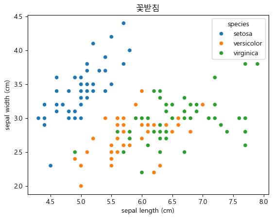
plt.title("꽃잎")
sns.scatterplot(data=iris_df, x="petal length (cm)", y="petal width (cm)", hue="species")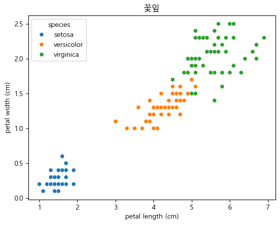
sns.pairplot(data=iris_df, hue="species")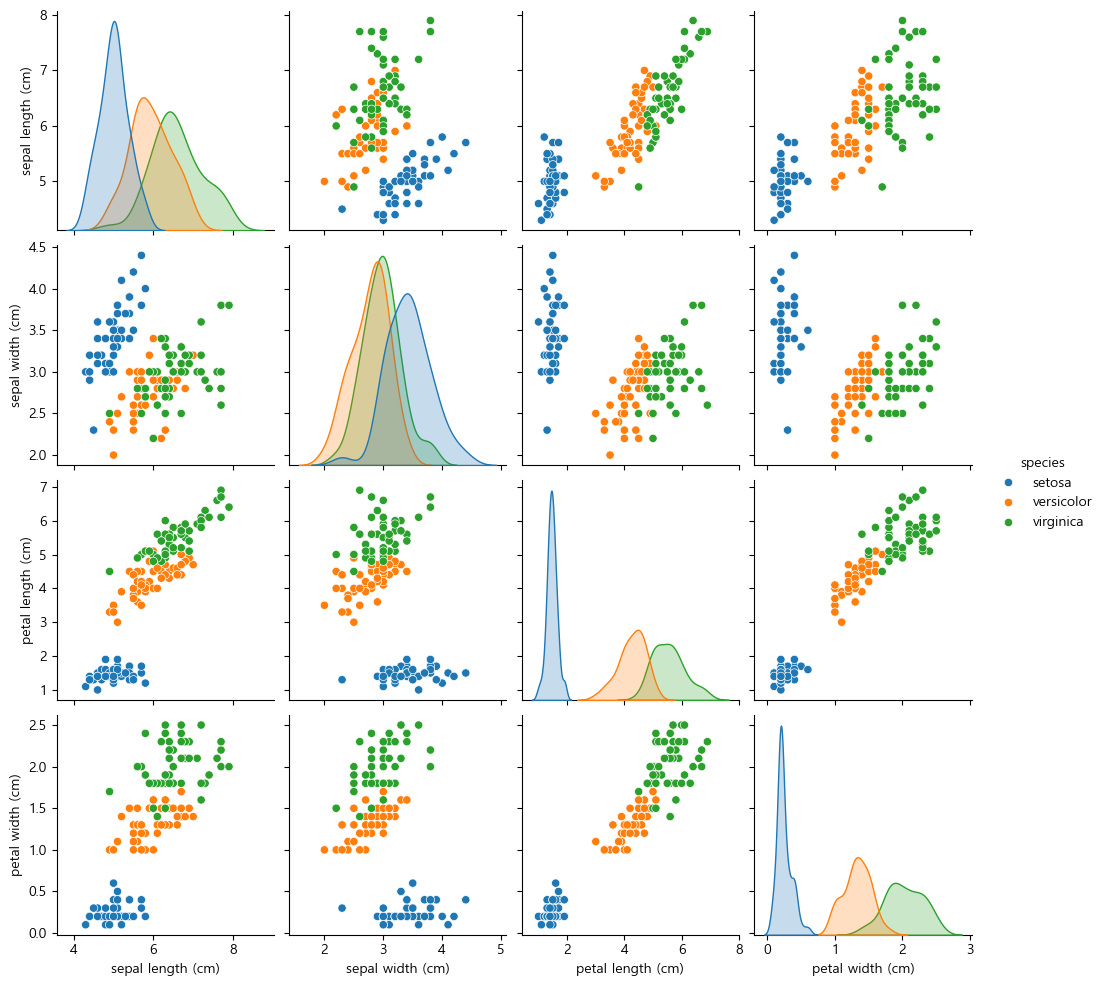
1.3. 통계적 검증
상관관계
이제 예측을 위해서는 각각의 열들간의 상관성이 있는지를 확인해야한다.
iris_df_num=iris_df.select_dtypes(include="number")
iris_df_num.corr().round(2)| sepal length (cm) | sepal width (cm) | petal length (cm) | petal width (cm) | |
|---|---|---|---|---|
| sepal length (cm) | 1.00 | -0.12 | 0.87 | 0.82 |
| sepal width (cm) | -0.12 | 1.00 | -0.43 | -0.37 |
| petal length (cm) | 0.87 | -0.43 | 1.00 | 0.96 |
| petal width (cm) | 0.82 | -0.37 | 0.96 | 1.00 |
1.4. 학습 및 평가 - PDA
1.4.1. 데이터 분할 및 변환
numpy로 넘어온것을 df로 바꿨는데 여기서 X와Y를 인덱스를 이용해서 뽑아도 된다.
그런데 이미 iris.data, iris.target과 같이 만들어져 있기 때문에
train_test_split을 사용해주면 된다.
순서는 다음과 같다.
- train_test_split으로 각각 학습데이터와 테스트데이터(_train, _test) 로 나누기
- Scalling으로 X값을 바꿔주기
2.1. StandardScaler 클래스의 생성자로 scaler라는 객체를 생성
2.2. fit함수에 X_train을 넣어 분산과 표준편차 구하고
2.3. transform함수에 이 구한 분산과 표준편차를 넣어서 z-score로 표준화를 한다.- 표준화를 마치면 이제 학습
3.1. KNeighborsClassifier 클래스의 생성자로 knn이라는 객체를 생성
3.2. fit함수에 스케일링한(표준화된) 값인 X_train_scale과 Y_train을 넣어 학습시키기- 이제 평가를하는데, 평가지표는 정확도다.
4.1. score함수에 표준화된 값인 X_train_scale과 Y_train을 넣은 학습한 정확도
4.2. score함수에 표준화된 값인 X_test_scale과 Y_test를 넣어 테스트가 잘 되었는지- 마무리로 예측
X_train, X_test, Y_train, Y_test=train_test_split(iris.data, iris.target, random_state=1234)

# 분산과 표준편차 구하기
scaler=StandardScaler()
scaler.fit(X_train)

# Z-score를 이용해 표준화
X_train_scale=scaler.transform(X_train)
X_test_scale=scaler.transform(X_test)
이제 학습을 해야한다.
knn=KNeighborsClassifier()
knn.fit(X_train_scale, Y_train)
이를 평가하면,
평가지표: 정확도
score는 정확도, 맞춘 데이터/전체 데이터
print("학습:", knn.score(X_train_scale, Y_train))
print("일반화:", knn.score(X_test_scale, Y_test))  # 테스트가 잘 되었는지
학습: 0.9642857142857143
일반화: 0.9473684210526315이제 예측을 할 것인데 이 부분이 중요하다.
데이터를 훈련시킬때, 데이터프레임이던가 넘파이로 데이터를 집어넣는데,
어제는 x는 df y는 series로 집어넣었음
그래서 예측을 할때도 df형태로 넣어줬음
그런데 이번에는 넘파이로 집어넣었기 때문에, numpy에 맞게 해야한다.
즉 예측에 데이터를 넣을때는 Numpy인지 DataFrame인지, 2차원인지, 1차원인지를 잘 봐서 맞춰서 넣어줘야한다.
new_data=scaler.transform([[5.1, 3.5, 1.4, 0.2]])
knn.predict(new_data)array([0])0이 나오므로 이는 setosa다.
1.4.2. ⭐ 오차행렬
분류모델 평가 방법
0. 오차 행렬(Confusion Matrix)
1. 정확도(Accuracy)
2. 정밀도(Precision)
3. 재현율(Recall)
4. F1-Score
지금까지 분류 모델에서 평가 방법으로 score라는 정확도를 썼는데, 이는 문제가 있다.
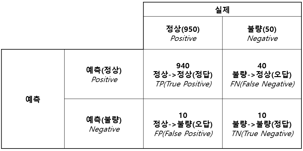
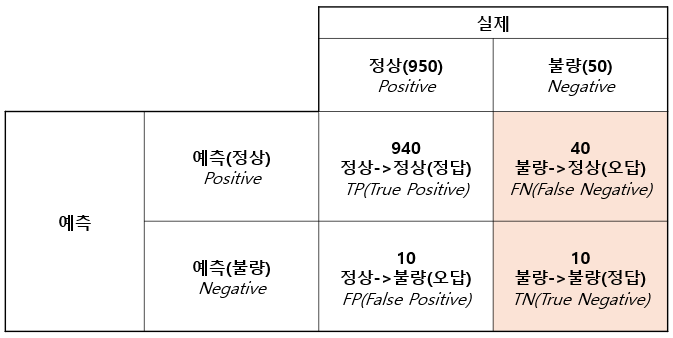
공장에서 정상인지 불량인지를 구분해야한다고 가정하자.
N=1000 개에서 정상은 950, 불량은 50으로 분류를 했는데,
이게 정상입장에서 봤을때,
950개중 940개를 정상을 정상으로 예측했고, 10개를 정상을 불량으로 예측했다.
그런데 불량입장에서,
50개중 40개를 불량을 정상으로 예측했고, 10개를 불량을 불량으로 예측했다.
그렇다면, 불량입장에서 불량을 정상으로 잘못맞춘거다.
그런데 정확도는 이런걸 감안하지 않는다.
그냥 950/1000 으로 95%의 예측률이라고 내놓는다.
이는 불량의입장으로 보면 아주 심각한 문제가 된다.
따라서 오차행렬(Confusion Matrix) 이라는 것이 있다.
오차행렬(Confusion Matrix)
이 표를 잘 기억하자.이를 오차행렬이라고 하며, 이 오차행렬을 기준으로 정확도와 정밀도, 재현율, F1-Score까지 다 계산할 수 있다.
- 정확도(Accuracy)
- 정밀도(Precision)와 재현율
정밀도와 재현율은 정상 기준과 불량 기준으로 나누어 본다.
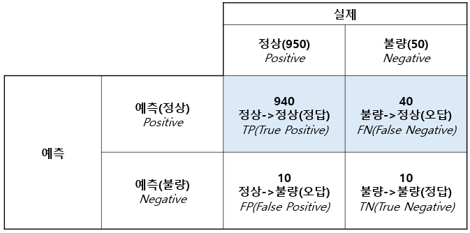
정상기준은 다음과 같다.
- 정상기준 Precision:
- 정상기준 Recall:
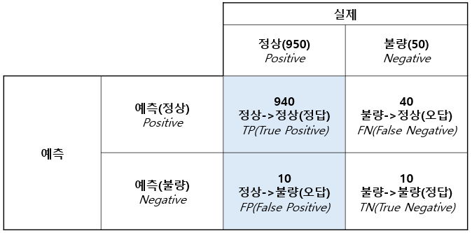
- 불량기준 Precision:
- 불량기준 Recall:
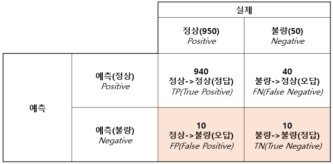
F1-Score
정상기준
불량기준
그리고 지금 이렇게 불량 기준 F1-Score가 28.6%라면, 불량의 감지를 잘 하지 못하는 것이기 때문에 좋지 않은 것이다.
이제 오차행렬로 쓸 수 있는 것들이 세토사(setosa, 0), 베시컬러(versicolor, 1), 버지니카(virginica, 2)다.
이는 라이브러리를 import해줘야 한다.
from sklearn.metrics import classification_reportY_test_predict=knn.predict(X_test_scaled)
print(classification_report(Y_test, Y_test_predict)) precision recall f1-score support
0 1.00 1.00 1.00 13
1 0.93 0.93 0.93 15
2 0.90 0.90 0.90 10
accuracy 0.95 38
macro avg 0.94 0.94 0.94 38
weighted avg 0.95 0.95 0.95 38이 마지막 support는 각 클래스의 실제 샘플의 수를 뜻한다.
그리고 Accuracy는 전체 38개의 샘플 중 95%를 정확하게 분류했다는 것을 의미하고,
macro avg는 각 클래스의 재현율, 정밀도 평균을 말하고,
wighted avg는 각 클래스의 데이터 수를 고려한 정밀도와 재현율 평균을 말한다.
-
세토사(Setosa, 0)
-
Precision: 1.00
세토사로 예측한 샘플 중 100%가 실제로 세토사다.
정확도가 100%다. -
Recall: 1.00
실제로 세토사인 샘플 중 100%를 모델이 정확하게 세토사로 예측했다. -
F1-score: 1.00
-
-
베시컬러 (Versicolor, 1)
-
Precision: 0.93
베시컬러로 예측한 샘플 중 93%가 실제로 베시컬러였다. -
Recall: 0.93
실제로 베시컬러인 샘플 중 93%를 모델이 정확하게 베시컬러로 예측했다. -
F1-score: 0.93
-
-
버지니카 (Virginica, 2)
-
Precision: 0.90
버지니카로 예측한 샘플 중 90%가 실제로 버지니카였다. -
Recall: 0.90
실제로 버지니카인 샘플 중 90%를 모델이 정확하게 버지니카로 예측했다. -
F1-score: 0.90
-
💪 퀴즈
Q1. sns.pairplot() 함수의 역할로 옳은 것은?
1) 변수 간의 상관 관계 시각화
2) 각 클래스 간의 평균 시각화
3) 각 변수의 분포 시각화
4) 변수 간의 관계를 여러 변수에 대해 한 번에 시각화
A1. 4
Q2. train_test_split() 함수의 역할로 옳은 것은?
1) 데이터를 스케일링한다.
2) 데이터를 학습용과 테스트용으로 분리한다.
3) 데이터를 시각화한다.
4) 데이터를 One Hot Encoding한다.
A2. 2
Q3. 모델 학습 후 평가할 때 사용되는 score() 함수는 무엇을 반환하나요?
1) 모델의 학습 시간
2) 정확도
3) 예측된 결과값
4) 예측 오류
A3. 2
Q4. 예측할 때,
scaler.transform([[5.1, 3.5, 1.4, 0.2]])와 같이 변환하는 이유는?
1) 데이터의 표준화하기 위해
2) 데이터를 카테고리형으로 변환하기 위해
3) 데이터를 훈련 데이터와 동일한 형식으로 변환하기 위해
4) 데이터를 범주형으로 변환하기 위해
A4. 1