[논문리뷰] On The Relationship Between Self-Attention and Convolution Layers

temp·2021년 8월 9일

AI Attention CNN paper-review transformer

Transformer / Vi-T / Attention and Convolution

목록 보기

1/6

Paper: ON THE RELATIONSHIP BETWEEN SELF-ATTENTION
AND CONVOLUTIONAL LAYERS
Code: github.com
Web: github.io

0. ABSTRACT

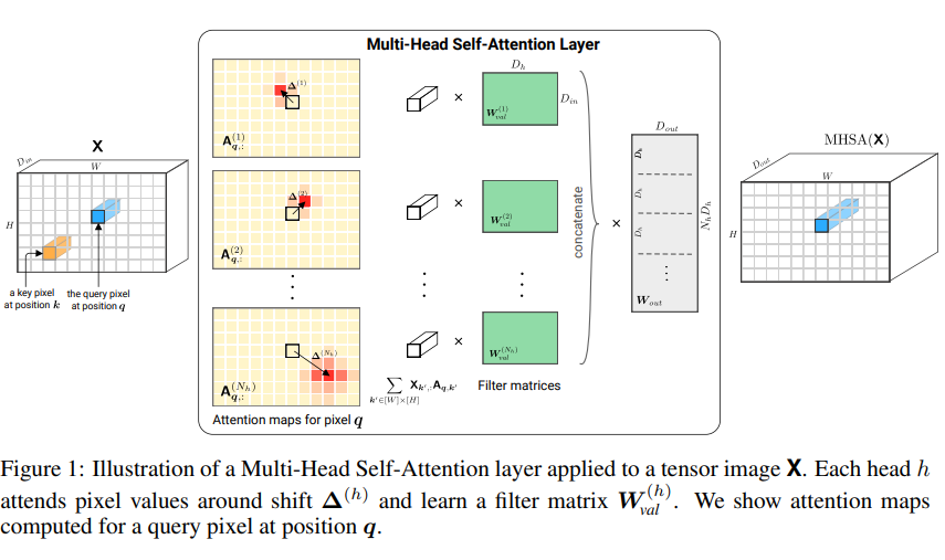
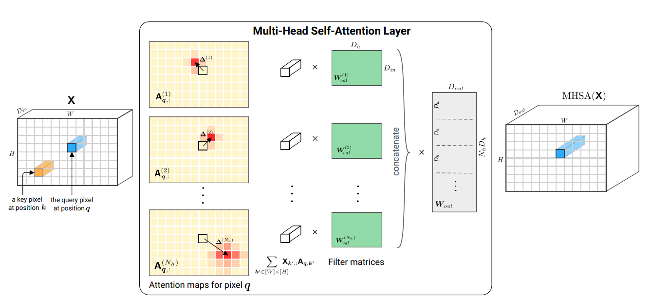
뒤에서 기술하겠지만, 위 그림에서 $D_{in}$ 는 image의 channels, $N_h$ 는 head 개수, $D_h$ 는 각 head의 차원입니다.

최근 attention 기법을 vision 분야에 통합하려는 시도들로 인해 백본 모델로 CNN을 사용하는 것을 재고하게 되었다. CNN이 장기적인 의존성을 처리하는 것을 돕는 걸 외에도, Ramachandran et al. (2019)는 attention이 완전히 convolution을 대체할 수 있고, vision task에서 SOTA 성능을 얻어낼 수 있음을 보여주었다. 즉, 자연스럽게 아래와 같은 질문이 생겨난다.

학습된 attention layer는 convolutional layer와 비슷한 역할을 하는가?

본 연구는 attention layer가 convolution를 수행할 수 있음을 보여주고, 실질적으로 학습도 같은 방식으로 수행된다는 것을 보여줄 것이다. 특히, 우리는 충분한 수의 head를 갖는 multi-head self-attention layer가 어떠한 convolutional layer 만큼이나 표현력 있다는 사실을 증명할 것이다. 우리의 numerical한 실험들도 self-attention layer 또한 CNN layers와 유사하게 pixel-grid patterns을 따른다는 것을 보여준다.

1. Introduction

Contributions

본 연구는 self-attention layer가 convolutional layers와 유사하게 행동한다는 이론적이고 실용적인 증거를 제공한다.

이론적인 관점에서, self-attention layers가 어떤 convolutional layers든 표현할 수 있다는 증명
- 구체적으로, relative positional encoding을 사용한 single multi-head self-attention layer는 어떤 convolutional layer든 간에 이를 표현하기 위해 re-parametrized될 수 있다.
attention-only 구조 중 첫 몇 개의 layer들이 매 query pixel 주변에서 grid-like한 pattern을 따른다는 결과(이론적인 관점과 비슷함).

Website에서는 self-attention이 localized position-based attention(lower layer)와 content-based attention(deeper layer)를 어떻게 탐색하는 지를 보여준다.

2. Background on Attention Mechanisms For Vision

본 단락에서는 self-attention layers의 수식과, positional encodings의 역할에 대해 다뤄보자.

2.1 The Multi-Head Self-Attention Layer

$\bold{X}\in \mathbb{R}^{T\times D_{in}}$ 를 각 $D_{in}$ dimension 내의 $T$ tokens으로 구성되어 있는 input matrix라 하자. NLP task에서는 각 token은 sentence 내 word겠지만, $T$ 개의 discrete objects를 갖는 어떠한 sequence에도 적용가능하다.

즉, Vison task에서는 $T$ 개의 pixel(with $D_{in}$ channel)을 갖는 sequence로 볼 수 있습니다.

self attention layer는 다음과 같이 모든 query token $t\in [T]$ 를 $D_{in}$ 차원에서 $D_{out}$ 차원으로 매핑시킬 수 있다.

이 때,
$T\times T$ 행렬 $\bold{A}:=\bold{X}\bold{W}_{qry}\bold{W}_{key}^{T}\bold{X}^{T}$ 를 attention scores로,
그리고 $softmax(\bold{A}_{t,:})$ 을 attention probabilities로 정의한다.

위 행렬은 단순히 input(embeddings) $X$ 가 query weight인 $W_{qry}$ 와 곱해지고, input $X$ 가 key weight인 $W_{key}$ 가 곱해진 다음, ( $D_k$ 차원에 projected된) query와 key가 곱해져 $(T,T)$ 차원의 attention score가 반환된 것으로 볼 수 있습니다. 그 후 input $X$ 가 value weight $W_{val}$ 와 곱해져 attention probabilities에 가중치가 부여되고, 최종적으로 $(T, D_{out})$ 의 output이 나옵니다.

즉, 이 self attention layer는
query matrix인 $D_{in}\times D_k$ 차원의 $\bold{W}_{qry}$ ,
key matrix인 $D_{in}\times D_k$ 차원의 $\bold{W}_{key}$ ,
value matrix인 $D_{in}\times D_{out}$ 차원의 $\bold{W}_{val}$

에 의해 parametrized된다고 볼 수 있다.

간단히 기술하기 위해 residual connections, batch normalization, constant factor 등은 생략하였습니다. DETR, velog의 후반부를 참고하면 대략적으로 이 요소들이 어떻게 적용되는 지 볼 수 있습니다.

$softmax(\bold{A}_{t,:})_k=exp(\bold{A}_{t,k})/\sum_pexp(\bold{A}_{t,p})$ 입니다.

위 식(1)의 output dimension은 $1\times D_{out}$ 이 됩니다( $T$ 개의 token 중 $t$ 번째 token에 대한 식).

위 식에서 나타난 self-attention model의 중요한 특징은 reordering을 하더라도 값이 동일하다는 것이다. 다시 말하면, $T$ input token이 어떻게 셔플되는지와는 무관하게, same output을 반환한다. 이는 순서가 중요한 task에 활용할 때 문제가 생길 수 있다.

이런 한계를 완화하기 위해 positional encoding이 sequence 내 each token(또는 pixel in an image)에 대해 학습된다. 그 후, self-attention을 적용하기 전, token의 representation에 더해진다.

즉,

위의 식이,

이처럼 변한다.

$T\times D_{in}$ 차원의 $\bold{P}$ 는 각 position에 대한 embedding vector를 포함합니다. 더 일반적으로 말하자면, $\bold{P}$ 는 position의 vector representation을 반환하는 어떤 함수로도 대체할 수 있습니다.

※ 중요
이러한 positional encoding으로 인해 self-attention 매커니즘을 multiple heads로 복제해, 각기 다른 query, key, value matrices를 사용함으로써, input의 다른 parts에 집중할 수 있게 되었다.

multi-head self-attention에서, output dimension $D_h$ 를 갖는 $N_h$ heads의 output은 concat되고, 곧바로 projected되어 $D_{out}$ dimension으로 표현된다. 식으로 나타내면 아래와 같다.

$\bold{W}_{out}$ : $N_hD_h\times D_{out}$ 차원의 projection matrix
$\bold{b}_{out}$ : $D_{out}$ 차원의 bias term

역시나 $T$ token은 그대로 남아 있습니다. 즉, $concat[Self-Attention_h(\bold{X})]$ 는 $T\times N_hD_h$ 차원입니다.

2.2 Attention for Images

Conv-Layer

Convolutional layers는 images 관련 neural network를 구성하는 데 사실상 필수였다.
즉, $W\times H\times D_{in}$ 차원의 $\bold{X}$ 를 image tensor라 할 때( $W$ :width, $H$ :height, $D_{in}$ : channels),
convolutional layer의 pixel $(i,j)$ 에 대한 output은 아래와 같이 주어진다.

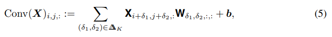
$\bold{W}$ : $K\times K\times D_{in}\times D_{out}$ 차원의 weight tensor
$\bold{b}$ : $D_{out}$ 차원의 bias vector

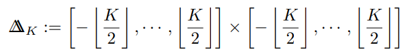
$\vartriangle_K$ : image를 $K\times K$ kernel로 convolving할 때 생길 수 있는 모든 shifts의 set

2D Image

다음으로는, 어떻게 self-attention이 1D sequence에서 images로 적합될 수 있는지 살펴볼 것이다.
tokens이 아닌 images라면, 우리는 query와 key pixels $\bold{q}, \bold{k} \in [W]\times [H]$ 를 갖는다 따라서, input은 $W\times H\times D_{in}$ 차원의 tensor이며, 각 attention score는 query와 key를 연관짓는다.

$\bold{q},\bold{k}$ 둘 다 2차원이며, 가능한 픽셀 값(위치)들을 갖습니다.

1D의 case에 맞춰진 식을 유지하기 위해, 2D index vector를 사용해 notation과 slice tensors를 대강 정의해보자. 예를 들면, $\bold{p}=(i,j)$ 일 때, $\bold{X}_{\bold{p}, :}$ 와 $\bold{A}_{\bold{p}, :}$ 를 $\bold{X}_{i,j,:}$ 와 $\bold{A}_{i,j,:,:}$ 를 나타내기 위해 사용한다. 이런 notation을 사용한다면, pixel $\bold{q}$ 에서의 self attention layer output은 아래와 같이 쓰여질 수 있다.

즉, 하나의 pixel $q$ 를 query로 여기고, 그 때의 attention 값은 가능한 모든 pixel $p$ 를 key로 여겨 연산합니다.

이는 multi-head case에도 그대로 적용된다.

기존의 $t$ 번째 token에 대한 attention 값을, $q$ 번 째 pixel에 대한 attention 값으로 대체합니다(query).

사실, 보다 나은 직관적인 이해를 위해 기존의 Transformer("Attention is all you need")를 먼저 이해하는 것이 좋습니다. 간단히 이해하기 위해 다른 분이 작성한 정리 글을 참고해도 될 듯 합니다.

2.3 Positional Encoding For Images

transformer-based 아키텍처에 쓰이는 positional encodings에는 absolute와 relative로 두 종류가 있다.

absolute encodings

absolute encodings을 사용하면, (fixed or learned) 벡터 $\bold{P}_{\bold{p},:}$ 가 각 pixel $\bold{p}$ 에 할당된다. 그 후, attention score의 연산(위의 식 (2))은 아래와 같이 분해될 수 있다.

이 때, $\bold{q}, \bold{k}$ 는 각각 query pixel, key pixel이다.

relative positional encodings

relative positional encoding은 Dai et al. (2019)에 의해 도입되었다. 메인 아이디어는 key pixel의 absolute position 대신 query pixel과 key pixel 간의 position difference만을 고려하는 것이다.

query pixel은 우리가 representation을 위해 연산하는 픽셀이고, key pixel은 우리가 주의를 기울이는 픽셀입니다. 사실 self-attention이기 때문에 둘을 구분하는 게 약간은 직관과 어긋나긴 합니다만(token attent itself..).

식은 아래와 같이 쓸 수 있다.

이 방식으로, attention score는 오직 shift $\bold{\delta}:=\bold{k}-\bold{q}$ 에만 의존한다. 위에서, 학습될 수 있는 벡터 $u, v$ 는 각 head에 대해 유니크하며, 모든 shift $\bold{\delta}$ 에 대해, relative positional encoding $\bold{r}_{\bold{\delta}}\in \mathbb{R}^{D_p}$ 는 모든 layer와 모든 head에서 공유된다.
또한, 여기서 key weights는 아래와 같이 두 종류로 나눠진다.

$\bold{W}_{key}$ : input과 관련됨
$\hat{\bold{W}}_{key}$ : pixel들의 상대적인 위치와 관련됨

3. Self-Attention as A Convoluitonal Layer

본 단락에서는 multi-head self-attention layer가 convolutional layer를 대체하기 위한 충분 조건을 증명합니다.

-위에 대한 증명이 주를 이루기 때문에 본 블로그에는 나타내지 않았습니다.

4. Experiments

4.1 Implementation Details

우리는 6개의 multi-head self-attention layers로 구성된 fully attentional model을 구성했다. 2019년에 Beelo et al.에 의해 attention features를 convolutional features와 결합하는 것이 성능 개선에 도움된다는 것이 밝혀졌지만, 본 연구에서는 SOTA 성능에 목표를 두지 않고, Standard ResNet18과 비교를 하는 데 중점을 두었다.

attention coefficient tensor는 input image의 사이즈에 맞게 정사각형으로 커지기 때문에, full attention은 큰 image에 적용될 수 없다(그래서 $2\times 2$ invertible down-sampling(Jacobsen et al., 2016)을 사용). input image의 고정된 size의 representation은 last layer representation의 average pooling으로 연산되며, 그 후 linear clssifier에 투입된다.

4.2 Quadratic Encoding

우선, 3장(생략)에서 도입된 relative position encoding을 사용하면 attention layers가 convolutional layers처럼 행동하게끔 학습될 수 있다는 것을 보여주려 한다. 우리는 ResNET 구조에 주로 쓰이는 $3\times 3$ kernel과 동등하게끔 각 layer마다 9개의 attention heads를 사용해 학습한다.

각 head $h$ 의 attention 중심은 특정 식에 따라 초기화됩니다.

아래의 그림(Figure 3)은, heads의 최초 위치가 학습에 따라 어떻게 변하는 지를 보여준다(at layer 4).

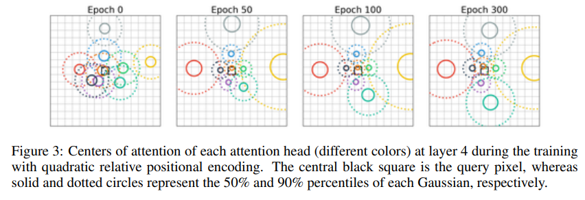
최적화 후에, heads는 query pixel 주변에 grid를 형성하면서, image에 특정 pixel위에 있음을 볼 수 있다.

즉, images에 적합된 Self-Attention이 queried pixel 주변의 convolutional filters를 학습한다는 직관이 확인되었다고 볼 수 있습니다.

아래의 그림(Figure 4)는 학습이 끝난 다음 모든 layer의 모든 attention head를 보여준다.

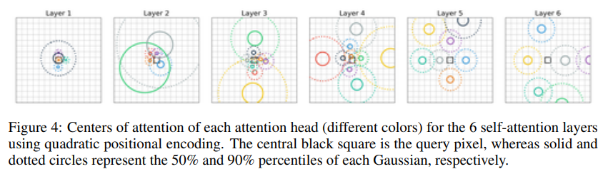
여기서, 초반의 few layers(layer 1, layer 2)는 local pattern에 집중하고, deep layers(layers 3-6)에서는 larger pattern에 집중하는 것을 볼 수 있습니다. 특히, queried pixel의 위치에서 멀리 떨어진 곳에 attention의 center를 위치시킵니다.

CNN의 filter와는 다르게, attention heads는 잘 겹치지 않으며, input space를 꽤나 광범위하게 다루는 것을 볼 수 있다.

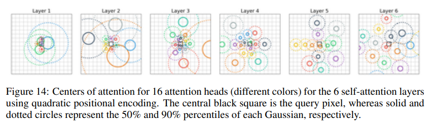
Attention heads를 16개로 키울 경우.

4.3 Learned Relative Positional Encoding

본 단락에서는 positional encoding을 중심적으로 다룰 예정이다.
우리는 $\lfloor D_p/2\rfloor$ position encoding vector를 각각의 행, 열 pixel shift에 대해 학습시킨다. 즉, key pixel $\bold{k}$ 와 query pixel $\bold{q}$ 의 relative positional encoding은 row shift embedding $\delta_1$ 과 column shift embedding $\delta_2$ 의 concat이다( $\delta=k-q$ ).

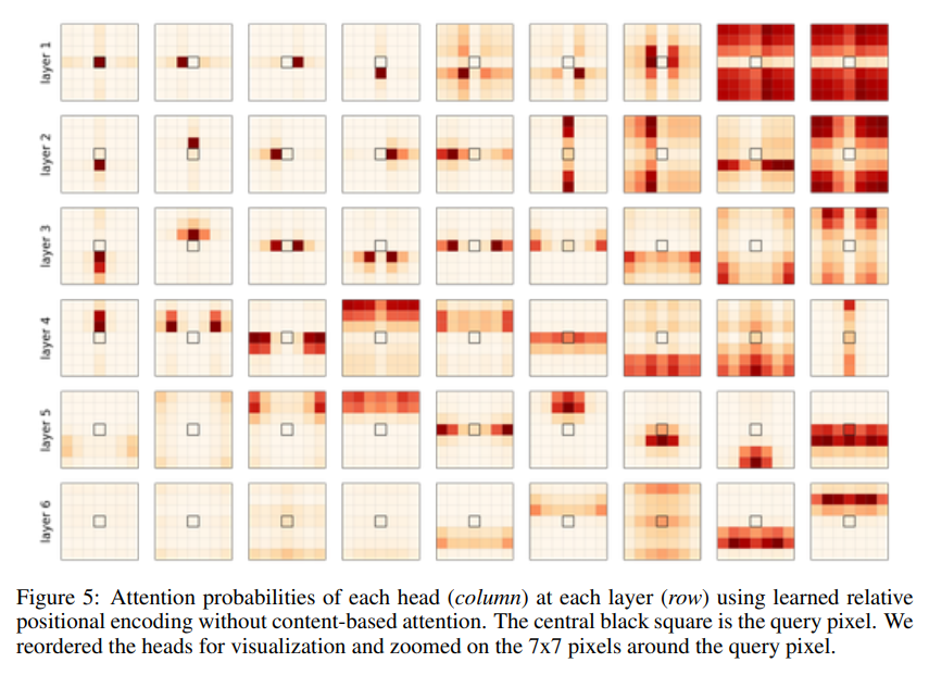
첫번째로, input data를 제거한 다음, 식(8)(positional encoding)에 따라서만 attention score를 연산했다. 각 head의 attention probabilities의 결과는 아래와 같다.

두번째로, attention score가 positional attention and content-based attention을 이용해 계산된, 현실성 있는 결과는 아래와 같다.

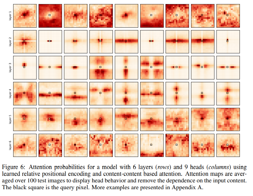
input image에 대한 의존성을 줄이고, 각각의 head에만 집중하기 위해 100 test image의 attention probabilities값을 평균 내어 시각화 하였습니다.

다만, 위 그림들의 의의는 3장에서 구성한 가설을 경험적으로 확인하는 것 뿐입니다.

결론적으로, 특정 self-attention layer(layer 2,3)는 convolutional kernel의 receptive filed를 모방하는 것처럼, query pixel에서 고정된 위치만큼 조금 떨어진 distinct pixel에 주의 집중한다는 것입니다.

query pixel을 image 내부에 sliding할 때 convolution과 multi-head self-attention 사이의 유사성이 더 잘 보인다.

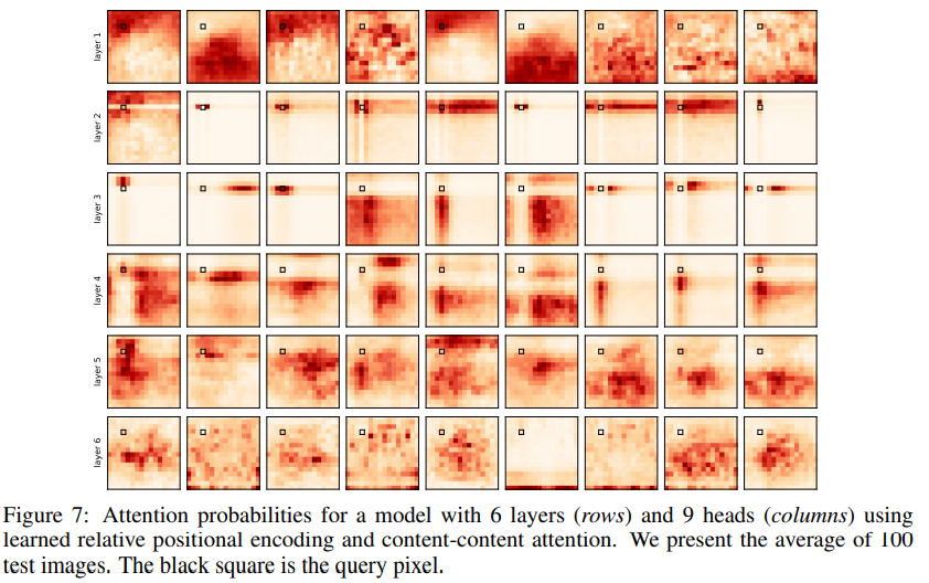
이를 Figure 6과 비교해봅시다.

layers 2 and 3의 attention pattern은 localized 됐을 뿐만 아니라, query pixel에서 고정된 위치만큼 떨어진 곳에 있다. 이는, image를 sliding하는 convolutional kernel(에 의해 생긴 receptive field)과 유사하다고 볼 수 있다..

Base paper

Prajit Ramachandran, Niki Parmar, Ashish Vaswani, Irwan Bello, Anselm Levskaya, and Jonathon
Shlens. Stand-alone self-attention in vision models. CoRR, abs/1906.05909, 2019

temp

다음 포스트