260203 [ Day 24 ] - ML, DL (2)

시작하며

오늘도 어제에 이어 통계학 공부를 이어갔다. ADsP 공부를 하면서 지겹도록 복습한 귀무가설에 대한 내용들과 아직도 적응이 안되는 여러 분포와 검정들에 대한 내용들을 배웠다.

코드로 확인

정규분포를 따르는 무작위 값 생성

• 평균 175, 표준편차 5인 정규분포를 따르는 가상의 키 데이터 생성(표본 수 = 5000)

heights = stats.norm.rvs(loc=175, scale=5, size=5000)

heights.mean()
# np.float64(175.12138663450918)
heights.std()
# np.float64(4.9588737381446055)

• 표본 수 = 500000

heights1 = stats.norm.rvs(loc=175, scale=5, size=500000)

heights1.mean()
# np.float64(175.0016360108597)
heights1.std()
# np.float64(4.9991504073228725)

부트스트래핑 코드

np.random.seed(1234)

avgs = pd.Series()

for i in range(1000):
    smpl = np.random.choice(a=heights, size=100, replace=True)
    avgs.loc[i] = smpl.mean()

avgs.describe().round(2)
# count    1000.00
# mean      175.10
# std         0.49
# min       173.19
# 25%       174.76
# 50%       175.10
# 75%       175.45
# max       176.69
# dtype: float64

정규분포 확률밀도

• 정규분포 확률밀도 함수(PDF)
  • $f(x) = \frac{1}{(\sqrt2\pi \times \sigma)} \times e^{- \frac{(x-\mu)^2}{2\sigma^2}}$
  • $\mu$ : 평균(분포 중심)
  • $\sigma$ : 표준편차(분포 퍼짐)
• 가능도 : 주어진 데이터가 특정 모수 $(\mu, \sigma)$ 에서 나올 확률
  • 데이터가 평균 분포 중심 근처 → 높은 가능도
  • 데이터가 평균 분포 꼬리 쪽 → 낮은 가능도
• 최대가능도 추정(MLE) : 관측 데이터를 가장 잘 설명하는 모수를 찾는 과정
  • 가능도 = $\prod f(xi)$ (각 데이터 확률 곱)
  • Log 가능도 = $\sum log f(xi)$ (계산 편의)
    • 진수가 0 ~ 1 = 로그값 음수로 출력
  • Log 가능도 최대화 = 비용함수 최소화
  • 미분 = 0 지점 → 최적 $\mu, \sigma$ 추정

stats.norm.pdf(x=175, loc=175, scale=15)
# np.float64(0.02659615202676218)

stats.norm.pdf(x=175, loc=175, scale=10)
# np.float64(0.03989422804014327)

stats.norm.pdf(x=175, loc=175, scale=5)
# np.float64(0.07978845608028654)

stats.norm.pdf(x=[169, 173, 175, 178, 182], loc=175, scale=5)
# array([0.03883721, 0.07365403, 0.07978846, 0.06664492, 0.02994549])

# 각 데이터 확률 곱
stats.norm.pdf(x=[169, 173, 175, 178, 182], loc=175, scale=5).prod()
# np.float64(4.5549448486331744e-07)

# 로그 가능도
np.log(stats.norm.pdf(x=[169, 173, 175, 178, 182], loc=175, scale=5)).sum()
# np.float64(-14.601882228193865)

# 로그 가능도 loc 비교
np.log(stats.norm.pdf(x=[169, 173, 175, 178, 182], loc=185, scale=5)).sum()
# np.float64(-23.80188222819387)

• 확률밀도곡선 시각화

x = range(125, 226)
y1 = stats.norm.pdf(x=x, loc=175, scale=15)
y2 = stats.norm.pdf(x=x, loc=175, scale=10)
y3 = stats.norm.pdf(x=x, loc=175, scale=5)

sns.lineplot(x=x, y=y1, label='Scale: 15')
sns.lineplot(x=x, y=y2, label='Scale: 10')
sns.lineplot(x=x, y=y3, label='Scale: 5')

plt.legend()

plt.show()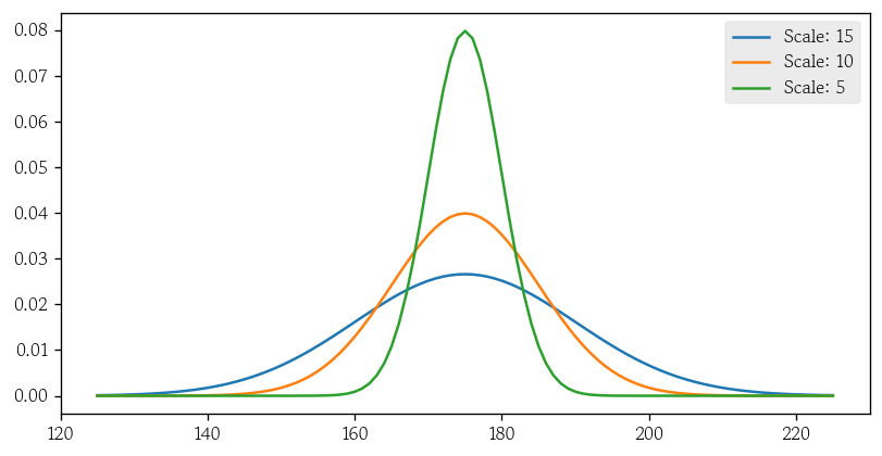

정규분포 누적확률

stats.norm.cdf(x=185, loc=175, scale=15)
# np.float64(0.7475074624530771)

stats.norm.cdf(x=185, loc=175, scale=10)
# np.float64(0.8413447460685429)

stats.norm.cdf(x=185, loc=175, scale=5)
# np.float64(0.9772498680518208)

cdfs = stats.norm.cdf(x=[165, 185], loc=175, scale=5)
np.diff(cdfs)
# array([0.95449974])

정규분포 확률변수값

stats.norm.ppf(q=0.748, loc=175, scale=15)
# np.float64(185.02313949588586)

stats.norm.ppf(q=0.841, loc=175, scale=10)
# np.float64(184.9857627061566)

stats.norm.ppf(q=0.977, loc=175, scale=5)
# np.float64(184.9769665508391)

rvs(Random Variates) : 난수 생성
pdf(Probability Density Function) : 확률밀도함수(연속형)
cdf(Cumulative Distribution Function) : 누적분포함수
ppf(Percent Point Functio) : x값 반환

왜도와 첨도

• 왜도 : 확률밀도곡선이 한 쪽으로 치우친 정도
  • 정규분포하는 데이터의 왜도는 0
  • 표본 왜도가 +-2일 때 정규분포한다고 판단
  • 왜도 > 0 : 오른쪽으로 꼬리가 긴 분포
  • 왜도 < 0 : 왼쪽으로 꼬리가 긴 분포

stats.skew(heights)
# np.float64(-0.03668062034777025)

• 첨도 : 봉우리의 뾰족한 정도
  • 정규분포하는 데이터의 첨도는 3
  • 표본 첨도가 1 ~ 5일 때 정규분포한다고 판단
  • stats.kurtosis : 내부적으로 3을 빼서 정규분포하는 데이터의 첨도를 0으로 반환

stats.kurtosis(heights)
# np.float64(-0.07067499523641407)

정규성 검정

• 데이터가 정규분포한다는 가정을 만족하는지 여부를 확인
  • 대표적으로 샤피로-윌크 검정과 앤더슨-달링 검정이 있음
• 샤피로-윌크 : 표본 데이터를 오름차순 정렬하고 표준정규분포에서 추출한 순위 통계량과의 상관계수를 통해 정규성 확인
  • N : 5000 까지만 가능
  • 귀무가설 : 데이터가 정규분포를 따른다
  • 대립가설 : 데이터가 정규분포를 따르지 않는다
• 앤더슨-달링 : 표본 데이터가 특정 확률분포에서 추출되었는지를 확인하며 정규성 검정에 사용
• statistic = 검정통계량
• pvalue = 유의확률

stats.shapiro(heights)
# ShapiroResult(statistic=np.float64(0.9995954653825436), pvalue=np.float64(0.40487292793217))

np.random.seed(1234)
heights = stats.norm.rvs(loc=175, scale=5, size=10000)

stats.anderson(heights)
# AndersonResult(statistic=np.float64(0.35265258232175256), critical_values=array([0.576, 0.656, 0.787, 0.918, 1.092]), significance_level=array([15. , 10. ,  5. ,  2.5,  1. ]), fit_result=  params: FitParams(loc=np.float64(175.08063230023598), scale=np.float64(4.9761483416071846))
#  success: True
#  message: '`anderson` successfully fit the distribution to the data.')

정규화

• 두 변수의 스케일을 동일하게 맞추는 과정으로 대표적인 방법에는 min-max 정규화와 표준화가 있음
  • min-max 정규화 : 모든 값을 0 ~ 1의 값으로 변환(음수X)
    • $\frac{x-min}{max-min}$
  • 표준화 : 평균이 0, 표준편차가 1이 되도록 값을 조정(음수O)
    • $Z=\frac{x - \mu}{\sigma}$

그림(히스토그램, 커널밀도추정), Q-Q Plot
왜도, 척도 확인
샤피로-윌크 & 앤더슨-달링

표준정규분포

• 정규분포를 따르는 두 확률변수의 표준편차가 다르면 확률변수값의 크기를 비교하기 어렵지만 표준화하면 비교 가능
  • 확률변수값을 z-score로 변환하는 것
  • z-score = $\frac{x - \mu}{\sigma}$
  • z-score는 확률변수값이 평균(0)에서 표준편차 단위로 얼마나 떨어져 있는지를 나타냄

표준화 함수

def scale(x, loc, scale):
    return (x - loc) / scale

scale(x=185, loc=175, scale=15)
# 0.6666666666666666

scale(x=185, loc=175, scale=10)
# 1.0

scale(x=185, loc=175, scale=5)
# 2.0

scale(x=90, loc=75, scale=15)
# 1.0

scale(x=55, loc=40, scale=10)
# 1.5

이상치 탐지

• 표준화 진행

scaled = scale(x=heights, loc=175, scale=5)
scaled
# array([ 0.47143516, -1.19097569,  1.43270697, ..., -1.05246069,
    #    -0.4976931 , -0.2560062 ], shape=(10000,))

• 절대값 기준 표준편차 3보다 큰 값(이상치) 탐색

cond = np.abs(scaled) > 3
cond
# array([False, False, False, ..., False, False, False], shape=(10000,))

outliers = heights[cond]
outliers
# array([157.1824167 , 190.62817574, 190.54817675, 155.59550794,
#        158.61347962, 191.10284213, 158.83247735, 157.82590423,
#        159.91806595, 159.24619206, 190.00573485, 158.67898086,
#        157.0030016 , 158.68108413, 159.25844267, 191.43893949,
#        158.34281695, 155.70665632, 190.18821417, 159.73908333])

• 이상치 인덱스 탐색

locs = np.where(cond)
locs
# (array([  81, 1307, 1333, 1670, 2053, 2289, 3136, 3924, 4477, 4599, 4712,
#         5274, 5903, 7040, 7510, 7743, 8578, 8650, 9406, 9888]),)

• scatterplot 으로 시각화

plt.figure(figsize=(12, 4))
sns.scatterplot(
    x=range(10000), y=heights, fc='0.9', s=25
)
sns.scatterplot(
    x=locs[0], y=outliers, fc='red'
)
plt.axhline(
    y=175, linestyle='-', linewidth=1, color='0'
)
plt.axhline(
    y=160, linestyle='--', linewidth=1, color='red'
)
plt.axhline(
    y=190, linestyle='--', linewidth=1, color='red'
)
plt.show()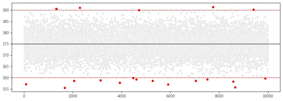

균일분포

• 확률변수의 실현값이 모두 같은 확률을 갖는 분포
• 이산형 균일분포는 확률변수가 가질 수 있는 값의 확률이 모두 같음
  • 시각화할 때 막대를 붙이지 않음
• 연속형 균일분포는 확률변수가 가질 수 있는 값의 확률이 구간(a, b)에서 모두 같음
  • 확률밀도함수 : $f(x) = \frac{1}{b - a}$

이항분포

• 시행 결과가 이진값인 베르누이 시행을 n번 실행할 때 성공 횟수의 분포
  • 확률질량함수 : $f(x) = \binom{n}{k} p^k (1-p)^{n-k}$
• 시행횟수(n)에 따라 분포 모양이 달라짐
  • 시행횟수가 커질수록 정규분포에 근사
• 모비율 검정 또는 로지스틱 회귀 분석에서 사용

푸아송 분포

• 단위 시간 또는 공간에서 어떤 사건이 발생하는 횟수를 나타내는 이산확률분포
  • 확률질량함수 : $f(x) = \frac{\lambda^k e^{-\lambda}}{k!}$ 단, $\lambda = n \times p$
  • 시행 횟수는 매우 크지만 발생확률이 아주 작은 이항분포

카이제곱 분포

• 독립적인 z-score의 제곱을 k개 더한 분포
  • 모분산을 추정할 때 사용
  • $\chi^2 = \sum_{i=1}^{k} z_i^2$
• 자유도(k)에 따라 분포 모양이 달라지며 자유도가 증가할수록 중심이 오른쪽으로 이동
• 교차분석 및 로지스틱 회귀 모형의 유의성 검정에서 사용

F 분포

• 카이제곱분포를 따르는 두 확률값을 각각의 자유도로 나눈 값의 비의 분포
• 분산분석에서 집단 간 변동과 집단 내 변동의 비가 1(등분산) 여부를 확인
• 선형 회귀 모형의 유의성 검정에서 사용

스튜던트 t분포

• 모분산을 모르고 표본의 크기가 작은 표본평균의 분포
  • 중심이 낮고 꼬리가 두꺼움
• 자유도는 n-1
• 표본이 커질수록 표준정규분포에 가까워짐
• 두 집답의 평균 차이가 서로 같은지 여부를 확인
• 선형 회귀계수의 유의성 검정에서 사용

확률분포 정리

• 이산확률분포
  • 균일분포
  • 베르누이분포
  • 이항분포
  • 푸아송분포
• 연속확률분포
  • 균일분포
  • 정규분포
  • 표준정규분포
  • t분포
  • 카이제곱분포
  • F분포

통계적 가설검정

통계적 가설검정의 이해

• 모수에 대한 주장을 표본 통계량을 이용해 검정함으로써 어떤 주장이 합당한 것인지를 판단하는 과정
  • 귀무가설(null hypothesis)과 대립가설(alternative hypothesis) 설정
  • 유의수준$(\alpha)$을 설정하면 양측검정과 단측검정 여부에 따라 기각역 결정
    • 보통 0.05 사용
  • 모집단을 대표하는 표본 통계량과 모수의 통계적 거리인 검정통계량을 계산
  • 검정통계량으로 유의확률을 계산하고, 유의확률이 유의수준보다 작으면 귀무가설을 기각

가설검정 관련 용어

검정통계량이 기각역에 위치하면 귀무가설을 기각

• 귀무가설 : 기각하기 위해 설정한 가설
• 대립가설 : 분석가가 채택하려는 가설
• 검정통계량 : 대립가설을 뒤받침해주는 모수와 표본 통계량의 통계적 거리
• 유의수준 : 참인 귀무가설을 기각하는 위험을 감내하는 수준
• 양측검정 : 기각역 크기는 양 극단에 0.025씩
• 단측검정 : 기각역 크기는 해당 방향으로 0.05

양측검정이 단측검정보다 임계값이 높음 → 귀무가설 기각 어려움

• 유의확률 : 귀무가설이 참이라는 가정 하에서 현재 관측된 검정통계량보다 극단적인 값이 나올 확률

검정력의 이해

• 제 1종 오류 : 귀무가설이 맞음 → 귀무가설 기각
• 제 2종 오류 : 대립가설이 맞음 → 귀무가설 기각 못함
• 검정력(power) : $1 - \beta$ > 0.8 이면 적절하다고 판단

가설검정의 종류

		조건	가설검정
일변량	연속형	대응 없음	단일표본 t-검정(모평균 검정)
일변량	연속형	대응 있음	대응표본 t-검정(차이의 모평균 검정)
일변량	범주형	단일표본	모비율 검정
일변량	범주형	두 표본	모비율 차이 검정
이변량	연속형-연속형	-	상관분석(무상관 검정)
이변량	연속형-범주형	범주 2개	독립표본 t-검정(모평균의 차이 검정)
이변량	연속형-범주형	범주 3개 이상	분산분석
이변량	범주형-범주형	-	교차분석(독립성 검정)

피어슨 상관분석

정규성 → 모수적 → 평균(값) 사용

• 두 연속형 변수에 상관관계가 있는지 측정
• 정규분포를 따르는 두 연속형 변수의 공분산을 각 표준편차로 나누어 표준화한 값(모수적 방법)
• -1 ≤ $\rho$ ≤ 1 을 만족
  • 절대값이 1에 가까울수록 강한 상관관계를 가짐
• 관련 함수는 상관계수와 유의확률을 반환

스피어만 순위상관분석

비정규성 → 비모수적 → 중위수(순서) 사용

• 이산형/순서형 변수의 의존성을 측정
• 한 변수의 순위가 증가할 때 다른 변수의 순위가 증가하는지 여부를 확인(순위를 고려한 비모수적인 방법)
• 피어슨 상관계수 공식에 두 변수의 순위 데이터로 계산
• 값이 1이면 한 변수의 순위가 증가할 때 다른 변수의 순위도 항상 같은 방향으로 증가한다는 것을 의미

모수적 방법과 비모수적 방법의 선택 기준

• 데이터가 정규성 가정을 만족하면 모수적 방법 사용
• 데이터가 정규성 가정을 만족하지 못하면 비모수적 방법 사용
• 실제 수집한 표본 데이터가 완벽하게 정규분포하는 경우는 거의 없음
  • 모집단이 정규분포하는 것으로 알려져 있고 표본의 크기가 충분할 때
  • 히스토그램이 좌우대칭의 종모양과 비슷하게 그려질 때
  • 왜도와 첨도로 정규분포한다고 판단 가능할 때
• 비모수적 방법 사용
  • 표본 크기가 매우 작아서 분포를 모르는 경우
  • 정규분포하지 않다는 것을 아는 경우
  • 데이터가 명목척도 또는 서열척도인 경우

피어슨 상관분석 코드

stats.pearsonr(x=df['Age'], y=df['Price'])
# PearsonRResult(statistic=np.float64(-0.796544729051927), pvalue=np.float64(5.8796109422549815e-279))

pg.corr(x=df['Age'], y=df['Price'])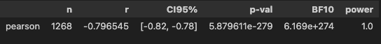

통계 보는 순서
p-val(CI95%) → r → power

lambda + apply

• lambda 사용

x = df['Age']

corr = lambda x: pg.corr(x=x, y=df['Price'])['p-val']

corr(x=df['Age'])
# pearson    5.879611e-279
# Name: p-val, dtype: float64

• apply 사용

df_num = df.select_dtypes(include=[int, float])
df_num.head()
# Price	Age	KM	HP	CC	Doors	Weight
# 0	13500	23	46986	90	2000	3	1165
# 1	13750	23	72937	90	2000	3	1165
# 2	13950	24	41711	90	2000	3	1165
# 3	14950	26	48000	90	2000	3	1165
# 4	13750	30	38500	90	2000	3	1170

df_num.apply(func=corr).lt(0.05)
#         Price	Age	  KM	  HP	  CC	  Doors	Weight
# pearson	True	True	True	True	False	True	True

t-검정 종류

구분	단일표본 t-검정	대응표본 t-검정	독립표본 t-검정
내용	표본 통계량과 모평균 비교	짝을 이루는 두 집단의 평균 비교	서로 독립인 두 집단의 평균 비교
기본 가정	정규성	정규성	독립성, 정규성, 등분산성
정규성 가정 만족X	윌콕슨 부호순위 검정	윌콕슨 부호순위 검정	윌콕슨 순위합 검정

• 독립성 : 수집 과정에서 확인

독립표본 t-검정

• 두 집단의 평균이 같은지 확인할 때 실행
• 두 집단 간의 변화량으로 두 집단의 평균 차이가 통계적으로 유의한지 확인
  • 두 집단의 평균 차이가 표준오차에 비해 충분히 크면 두 집단의 평균은 같지 않다고 판단
  • 작으면 두 집단의 평균은 같다고 판단

t-검정 자료구조

• 범주별 연속형 목표변수가 정규분포하거나 잔차가 정규분포 해야함

독립표본 t-검정의 가설 및 검정통계량

• 귀무가설 : $\mu_1 - \mu_2 = 0$ (두 집단의 모평균이 같음)
• 대립가설 : 두 집단의 모평균이 같지 않음
• 유의수준 : 0.05 → 양측검정
• 검정통계량 : $t = \frac{(\bar{X}_1 - \bar{X}_2) - (\mu_1 - \mu_2)}{\sqrt{s_p^2 \left(\frac{1}{n_1} + \frac{1}{n_2}\right)}}$
  • $\bar{X_1} - \bar{X_2}$ : 표본 평균의 차이
  • 모평균의 차이는 귀무가설에 의해 0이 됨
  • 분모는 두 표본평균의 표준오차이며 모분산의 불편추정량인 합동표본분산임
    • 두 표본분산이 같다는 가정

두 집단의 기술통계량 확인

pvt = pd.pivot_table(
    data=df,
    values='Price',
    index='MetColor',
    aggfunc=['count', 'mean', 'std']
)
pvt.columns = pvt.columns.droplevel(1)
pvt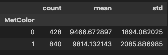

독립표본 t-검정의 가정

• 독립성, 정규성 및 등분산성 가정을 만족해야 함
  • 독립성 가정 : 두 집단 간 차이에 영향을 주는 외부 요인이 없어야 함
  • 실험 데이터는 무작위화를 통해 외부 요인을 상쇄 가능
  • 잔차는 정규분포하고 모분산이 같아야 함

정규성 검정

• t-검정 : 잔차의 정규성 가정을 만족해야 함
• dv : dependent variable(종속변수)

pg.normality(data=df, dv='Price', group='MetColor')
#          W	       pval	       normal
# MetColor			
# 1	       0.974755	7.062942e-11	False
# 0	       0.988074	1.430807e-03	False

등분산성 검정

• 정규성 가정을 만족하는 두 집단의 등분산성 검정 실행
  • 현실에서는 정규성 검정을 만족하는 데이터를 구하기 힘들어 만족한다고 가정하기도 함

pg.homoscedasticity(data=df, dv='Price', group='MetColor')
#              W	    pval	  equal_var
# levene	5.761315	0.016526	False

t-검정

등분산 : t-검정
이분산 : Welch의 t-검정

• correction : True 시 이분산, False 시 등분산

pg.ttest(x=y1, y=y2, correction=True)

맨-휘트니 U 검정

• 두 집단 분포 위치가 같은지 여부를 판단하는 비모수적인 검정

pg.mwu(x=y1, y=y2)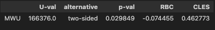

마치며

워낙 많은 내용이기도 하고, 어려운 내용들이라 공부를 하는데 체력을 너무 많이 쓴 느낌이 들었다. 자격증 공부를 하면서 조금씩 익숙해진 내용들이긴 해도 자세히 파고드니까 여전히 어려웠다. 내일은 알고리즘 문제 관련 특강이 있어서 한숨 돌리면서 자격증 공부와 복습을 꾸준히 해야겠다.