시작하며
오늘부터 새로운 파트인 머신러닝과 딥러닝 심화 파트에 들어갔다. 본격적으로 머신러닝과 딥러닝에 대해 공부하기 전에 필요한 통계학에 대해 더 깊게 배운 뒤에 머신러닝과 딥러닝을 배울 것 같다. 이전 파트에서도 가볍게 통계학을 다루긴 했는데 이번에는 조금 더 복잡하고 어려운 내용을 다뤘다.
기술통계 분석
통계 개요
- 통계 : 데이터를 수집, 요약 및 추론 등을 통해 분석하는 방법론
- 데이터 수집은 표본 추출, 요약은 기술통계, 추론은 모수 추정을 의미
- 주요 용어
- 모집단 : 조사 대상이 되는 개체의 전체 집합이며 유한하거나 무한함
- 모수 : 모집단의 특성을 나타내는 확정된 값(상수)
- 표본 : 모집단에서 추출한 부분 집합이며 모집단을 대표해야 함
- 통계량 : 표본의 수치를 요약한 값
표본 추출 프로세스
모집단 정의 → 프레임 확보 → 표본 추출 방법 결정 → 표본 크기 결정 → 표본 추출
표본 추출 방법
- 확률적 표본 추출
- 단순 무작위 표본 추출 : 모집단에서 선택될 확률이 같다는 가정 하에 무작위로 표본 추출
- 계통적 표본 추출 : 모집단에서 무작위 시작점부터 일정한 간격으로 선택하여 표본 추출
- 층화 표본 추출 : 모집단을 동질적 집단으로 나누고 각 집단에서 무작위로 표본 추출
- 집략 표본 추출 : 모집단을 이질적 집단으로 나누고 무작위로 선택한 집단을 전수 조사
- 비확률적 표본 추출(도메인 지식 필수)
- 편의 표본 추출 : 사전에 정한 표본 크기를 충족할 때까지 접근하기 쉬운 표본 추출
- 판단 표본 추출 : 연구자 주관 하에 모집단에 대한 대표성이 있다고 판단하는 표본 추출
- 할당 표본 추출 : 모집단의 몇 개의 집단으로 나누고 집단에 할당한 크기만큼 표본 추출
- 눈덩이 표본 추출 : 연구자가 임의로 선정한 표본으로부터 추천받아 눈덩이 굴리듯 추적
기술통계
- 기술통계 : 데이터의 주요 특징을 빠르게 파악할 때 사용
- 주요 통계량
- 중심위치(대푯값) : 평균, 절사평균, 중위수, 최빈값
- 상대위치(분위수) : 백분위수, 십분위수, 사분위수, 최솟값, 최댓값
- 변동성(산포) : 범위, 사분범위, 분산, 표준편차, 변동계수, 중위수절대편차
데이터 척도의 종류
- 범주형(질적 자료)
- 명목 척도
- 값 사이에 순서가 없음
- 등호와 부등호 비교만 의미가 있음
- 성별, 혈액형 등
- 서열 척도
- 값 사이에 순서는 있지만, 간격은 불명확
- 등호, 부등호 및 순서 비교에 의미가 있음
- 만족도, 학년, 등급 등
- 명목 척도
- 이산형(양적 자료)
- 등간 척도
- 간격은 일정하지만, 0 = 있는 것
- 덧셈과 뺄셈은 가능하지만 비율(몇배)은 불가
- 온도, 연도 등
- 비율 척도
- 간격이 일정하고, 0 = 없는 것
- 사칙연산이 가능하므로 비율 계산 가능
- 무게, 키, 소득, 나이 등
- 등간 척도
| 구분 | 동일 여부(=, ≠) | 순서 있음(<, >) | 간격 일정(+-, 평균) | 절대 0 존재(X, %) |
|---|---|---|---|---|
| 명목척도 | O | X | X | X |
| 서열척도 | O | O | X | X |
| 등간척도 | O | O | O | X |
| 비율척도 | O | O | O | O |
데이터 분석
- 주제 = Y변수(종속변수, 타겟변수, 내생변수)
- 객관적으로 측정가능
- 값이 없을 경우 → 조작적 정의
- 상관관계가 있는 변수 나열(가설수립) → 도메인 전문성 필요
평균
- 평균 : 연속형 변수의 원소를 모두 더한 값을 원소 개수로 나눈 값
- 전체 데이터를 포함하므로 극단값에 민감하게 영향을 받는 단점이 있음
df['Price'].mean()
# np.float64(9690.232941176471)skipna속성으로 결측값을 제외한 평균 반환
nums = pd.Series([1, np.nan, 2])
nums.mean()
# np.float64(1.5)
절사평균
- 절사평균 : 연속형 변수의 양 극단에서 일부를 제외한 평균
stats.trim_mean(df['Price'], proportiontocut=0.1)
# np.float64(9584.380019588638)- 평균보다 값이 낮아짐 → 높은 극단값이 존재
중위수
- 중위수 : 연속형 변수를 오름차순 정렬했을 때 정가운데에 위치한 값
- 원소 개수가 홀수면 정가운데 원소
- 원소 개수가 짝수면 가운데 두 원소의 평균
- 극단값에 강건한 통계량
- 극단값이 많은 데이터는 평균과 중위수를 함께 확인
df['Price'].median()
# np.float64(9450.0)
최빈값
- 최빈값 : 이산형(정수, 범주, 문자열) 변수에서 도수가 가장 높은 원소
df['FuelType'].mode()
# 0    Petrol
# Name: FuelType, dtype: object- 변수의 도수 확인
df['FuelType'].value_counts()
# FuelType
# Petrol    1129
# Diesel     129
# CNG         17
# Name: count, dtype: int64- 상대도수 확인
df['FuelType'].value_counts(normalize=True)
# FuelType
# Petrol    0.885490
# Diesel    0.101176
# CNG       0.013333
# Name: proportion, dtype: float64
분위수
- 분위수 : 오름차순 정렬한 연속형 변수를 n 등분하는 경계값
- 사분위수
df['Price'].quantile(np.linspace(0, 1, 5))
# 0.00     4350.0
# 0.25     8250.0
# 0.50     9450.0
# 0.75    10950.0
# 1.00    15950.0
# Name: Price, dtype: float64- 십분위수
df['Price'].quantile(np.linspace(0, 1, 11))
# 0.0     4350.0
# 0.1     7250.0
# 0.2     7950.0
# 0.3     8500.0
# 0.4     8950.0
# 0.5     9450.0
# 0.6     9950.0
# 0.7    10500.0
# 0.8    11456.0
# 0.9    12500.0
# 1.0    15950.0
# Name: Price, dtype: float64
최솟값과 최댓값
df['Price'].min()
# np.int64(4350)

df['Price'].max()
# np.int64(15950)quantile사용
df['Price'].quantile([0, 1])
# 0.0     4350.0
# 1.0    15950.0
# Name: Price, dtype: float64agg사용
df['Price'].agg(func=['min', 'max'])
# min     4350
# max    15950
# Name: Price, dtype: int64
범위와 사분범위
- 범위 : 연속형 변수의 최댓값과 최솟값의 간격
df['Price'].max() - df['Price'].min()
# np.int64(11600)quantile과diff사용diff: 인접한 두 원소 간의 차이를 반환
df['Price'].quantile([0, 1]).diff().iloc[-1]
# np.float64(11600.0)- 사분범위 : 연속형 변수의 3사분위수와 1사분위수의 간격
df['Price'].quantile([0.25, 0.75]).diff().iloc[-1]
# np.float64(2700.0)
분산
- 분산 : 개별 관측값이 중심에서 떨어져 있는 정도(편차 제곱의 평균)
- 편차 : 개별 관측값이 중심(평균)에서 떨어져 있는 크기(관측값 - 중심(평균))
- 표본 분산은 편차 제곱의 평균을 계산한 것이며, 불편추정량이 되도록 n - 1로 나눔
- 분산이 작을수록 개별 관측값이 평균에 밀집해 있다고 판단
ddof는 degree of freedom이며, 1을 지정하면 편차 제곱합을 n-1로 나눔
df['Price'].var()
# np.float64(4120265.326386555)
df['Price'].var(ddof=0)
# np.float64(4117033.7457384085)- 넘파이에서의 분산
ddof기본값 = 0
np.var(df['Price'])
# np.float64(4117033.7457384085)
표준편차
- 표준편차 : 개별 관측값이 중심에서 떨어져 있는 정도
- 분산은 편차를 제곱했으므로 원래 변수의 측정 단위와 달라짐
- 표준편차는 분산의 양의 제곱근이며, 원래 변수와 측정 단위가 같아짐
- 개별 관측값이 중심에서 떨어져 있는 정도를 파악할 때 표준편차를 확인
- 표준편차도 작을수록 개별 관측값이 편귱에 밀집해 있다고 판단
df['Price'].std()
# np.float64(2029.8436704304484)
변동계수
- 변동계수 : 표준편차를 평균으로 나눈 값
- 측정 단위가 다른 변수 간 변동성을 비교할 때 사용하므로 상대표준편차라고도 함
- 변동계수는 측정단위가 서로 다른 변수를 비교할 때 사용
- 상대적인 변동성을 사용
- 상대표준편차는 변동계수에 100을 곱해 백분율로 나타낸 값이며, 주로 실험과학에서 사용
- 측정의 정밀도에 초점을 맞춤
중위수절대편차
- 중위수절대편차 : 평균 대신 중위수를 사용
- 표준편차보다 강건한 통계량
- 편차 절대값의 중위수를 계산하고 모수 추정 상수 1.4826을 곱함
robust.mad(df['Price'])
# np.float64(2223.903327758403)
기술통계량 확인
- 평균과 중위수 비교
- 1사분위수 - 중위수, 3사분위수 - 중위수 비교(그래프 모양 유추 가능)
- 최솟값, 최댓값 확인
- 범주형 변수 기술통계량(원소 개수, 고유값 개수, 최빈값 및 최빈값의 도수)
df.describe(include=object)
#   FuelType	MetColor	Automatic
# count	1273	1273	1273
# unique	3	2	2
# top	Petrol	1	0
# freq	1128	842	1203
공분산
- 공분산 : 두 연속형 변수 간 상관관계의 방향을 나타내는 통계량
- x가 증가할 때 대응하는 y가 증가하면 공분산은 양수
- x가 증가할 때 대응하는 y가 감소하면 공분산은 음수
- x와 y의 측정 단위가 다를 수 있으므로 공분산은 상관관계의 방향만 확인
df['Age'].cov(df['Price'])
# np.float64(-22136.617857831003)- 연속형 변수 간 분산-공분산 행렬 확인
df.cov(numeric_only=True).round(2)
#           Price	Age	KM	HP	CC	Doors	Weight
# Price	4117054.19	-22136.62	-3.747196e+07	5977.21	17623.05	325.35	15746.20
# Age	-22136.62	187.56	1.711083e+05	-8.46	-210.17	-1.22	-102.32
# KM	-37471955.30	171108.28	1.285867e+09	-156932.02	2588046.91	467.42	359285.14
# HP	5977.21	-8.46	-1.569320e+05	172.01	-53.44	1.58	-41.74
# CC	17623.05	-210.17	2.588047e+06	-53.44	34010.01	23.36	5010.95
# Doors	325.35	-1.22	4.674200e+02	1.58	23.36	0.90	13.10
# Weight	15746.20	-102.32	3.592851e+05	-41.74	5010.95	13.10	1553.06
상관계수
- 상관계수 : 공분산을 각 변수의 표준편차로 나눈 것
- 상관계수는 두 연속형 변수 간 상관관계의 방향과 강도를 함께 나타냄
- 상관계수는 -1 ~ 1의 값을 갖는데 1에 가까울수록 강한 상관관계가 있다고 판단
- 데이터의 형태에 따라 피어슨 상관계수 또는 스피어만 순위상관계수를 계산
- 값의 상관관계 : 정규성(피어슨 상관계수)
- 순서의 상관관계 : 비정규성(스피어만 순위상관계수)
df['Age'].corr(df['Price'])
# np.float64(-0.7966182791038179)- 상관계수 행렬
df.corr(numeric_only=True)
#           Price	      Age	      KM	     HP	         CC	        Doors	  Weight
# Price	1.000000	-0.796618	-0.515009	0.224610	0.047096	0.168562	0.196920
# Age	-0.796618	1.000000	0.348422	-0.047075	-0.083213	-0.093670	-0.189588
# KM	-0.515009	0.348422	1.000000	-0.333686	0.391355	0.013703	0.254242
# HP	0.224610	-0.047075	-0.333686	1.000000	-0.022095	0.126925	-0.080759
# CC	0.047096	-0.083213	0.391355	-0.022095	1.000000	0.133181	0.689482
# Doors	0.168562	-0.093670	0.013703	0.126925	0.133181	1.000000	0.349477
# Weight	0.196920	-0.189588	0.254242	-0.080759	0.689482	0.349477	1.000000
상관관계 vs 인과관계
- 두 변수에 상관관계가 있다는 것이 인과관계가 있다는 것을 의미하지 않음
- 인과관계 : 원인 변수가 결과 변수에 영향을 주는 관계
- 상관관계는 두 변수가 함께 변하는 경향(직선)을 의미하며, 영향을 주고받는 관계를 의미하는 것은 아님
탐색적 데이터 분석
그래프 설정
- 기본 프리셋 설정
import seaborn as sns
import matplotlib.pyplot as plt

plt.rc(group='font', family='Gowun Batang', size=10)
plt.rc(group='figure', figsize=(8, 4), dpi=120)
plt.rc(group='axes', unicode_minus=False)
plt.rc(group='legend', frameon=True, fc='0.9', ec='0.9')- 그래프 크기 설정
plt.rc(group='figure', figsize=(4, 4))목표변수 분포 확인(히스토그램)
- 목표변수의 최솟값과 최댓값 확인
df['Price'].agg(func=['min', 'max'])- 목표변수로 히스토그램 그리기
sns.histplot(
    df, x='Price', binrange=[4000, 16000],
    binwidth=1000, facecolor='0.8'
)

plt.show()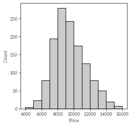
목표변수 분포 확인(커널 밀도 추정 곡선)
sns.kdeplot(
    df, x='Price',
    fill=True, color='0.8'
)

plt.axvline(df['Price'].mean())
plt.axvline(df['Price'].median(), color='red', linestyle='--')

plt.show()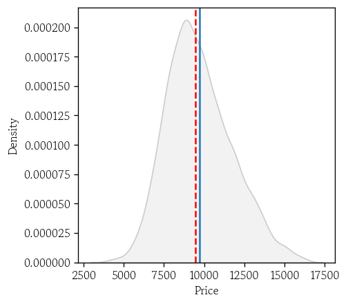
연속형 변수 간 상관관계 확인(히트맵)
corr = df.corr(numeric_only=True)
sns.heatmap(
    corr, annot=True, fmt='.2f',
    annot_kws={'size': 8},
    cmap='RdYlBu', linewidths=1
)

plt.show()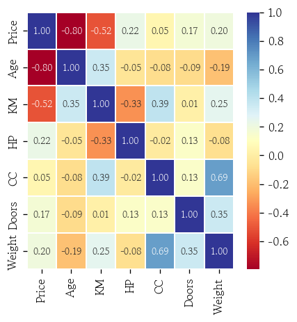
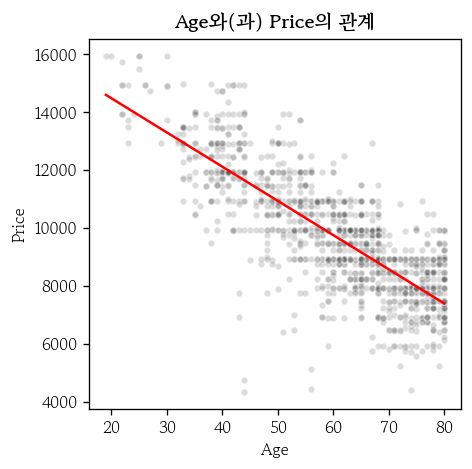
연속형 입력변수와 관계 확인(1)
hds.plot.regline(
    df, x='Age', y='Price'
)- 정규성
- 등분산성
- 단순 선형회귀식은 항상 점을 지남
- x축에서 더 멀리있는 이상치가 더 영향을 크게 줌
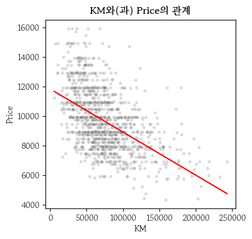
연속형 입력변수와 관계 확인(2)
hds.plot.regline(
    df, x='KM', y='Price'
)- 선형관계가 아닌경우
- 변환 : 로그, 제곱근 → Feature Engineering
- 나누기 : 일정 기준으로 모델을 나누기
- 많은 데이터를 설명할 수 있는 하나의 모델을 만드는 것은 쉽지 않음
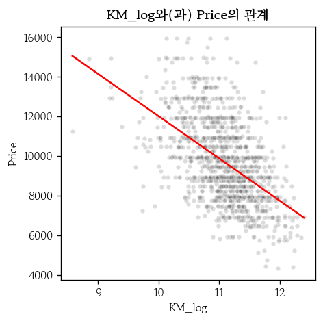
- 로그로 변환
df1 = df.copy()
df1['KM_log'] = np.log(df1['KM'])

hds.plot.regline(
    df1, x='KM_log', y='Price'
)
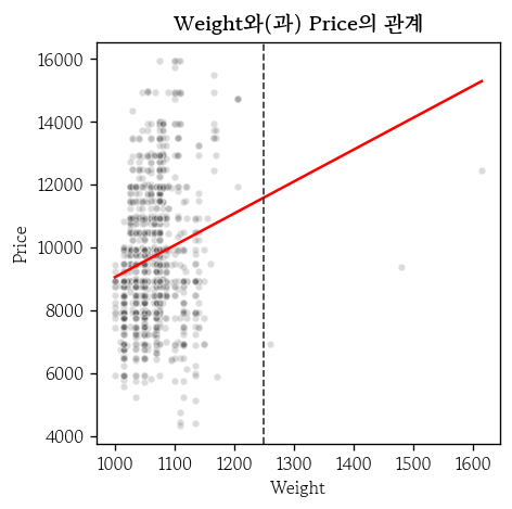
연속형 입력변수와 관계 확인(3)
hds.plot.regline(
    df, x='Weight', y='Price'
)

plt.axvline(
    x=1250, ls='--', lw=1, color='0.2'
)- 외삽 : 데이터 범위 밖
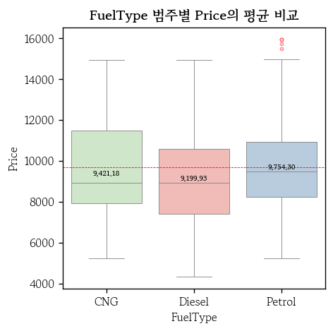
범주형 입력변수와 관계 확인(박스플롯)
hds.plot.box_group(
    df, x='FuelType', y='Price',
    palette='Pastel1'
)
불필요한 행 삭제
cond1 = df['Doors'].ne(2)
cond2 = df['Weight'].le(1250)

df = df.loc[cond1 & cond2, :]
df = df.reset_index(drop=True)
df.shape
외부 파일로 저장
df.to_pickle(): 데이터프레임 하나를 pickle 파일로 저장pd.to_pickle(obj, filepath_or_buffer): obj 매개변수에 지정한 파이썬 객체를 pickle 파일로 저장- 여러 객체를 하나의 pickle 파일로 저장
확률변수와 확률분포
집합과 원소
- 집합 : 어떤 조건을 만족하는 대상들이 모인 무리
- 원소 : 집합에 속한 대상 → 중복하여 표기 X
- 어떤 원소가 그 집합에 속하는지 여부를 명확하게 구분
- 일반적으로 알파벳 대문자로 표기하고 원소는 소문자로 표기
벤다이어그램
- 두 집합의 관계를 그림으로 표현한 것
확률의 개념
- 일정한 조건 하에서 어떤 사건이 우연하게 발생할 가능성의 정도를 0~1 사이의 실수로 나타낸 것
- 확률에 100을 곱한 백분율로 표기하기도 함
- 확률은 계산하는 방법에 따라 수학적 확률과 통계적 확률고 구분
- 수학적 확률 =
- 통계적 확률 =
- 시행 횟수를 반복 할수록 통계적 확률은 수학적 확률에 가까워짐
확률의 특징
- 표본 공간(S)의 확률은 1
주사위 한 번 던지기의 표본 공간
사건 A : 1, 3, 5
사건 B : 2, 4, 6
- 개별 사건이 발생할 확률
- 홀수인 사건 A의 확률 :
- 짝수인 사건 B의 확률 :
- 확률의 덧셈정리가 성립
- 배반사건이면 교집합이 없음
- 사건 A가 발생하지 않을 여사건의 확률
확률 관련 주요 용어
- 시행 : 실험 또는 관찰을 반복하여 결과물을 얻는 과정
- 표본 공간 : 시행에서 발생 가능한 모든 결과의 집합이며 보통 S로 표기
- 사건 : 사전에 정의한 조건을 만족하는 시행의 결과
조건부 확률
- 사건 A가 일어났을 때 사건 B가 일어날 확률
- 반대의 경우도 마찬가지
독립과 종속
- 독립사건 : 어떤 사건이 발생하는 것이 다른 사건의 발생에 영향을 주지 않는 것
- 많은 머신러닝 알고리즘에서 개별 관측값의 발생을 독립사건으로 가정
- 사건 A와 B가 독립일 때 두 확률의 곱은 교집합일 확률과 같음
- 독립이 아닌 경우(종속) 두 확률의 곱
- 조건부 확률 공식에서 분모를 양변에 곱한 식
베이즈 정리
- 사전확률과 가능도로부터 사후확률을 추정
- 사후확률 : 우리가 알고자 하는 확률
- 사건 B가 발생했을 때 사건 A의 확률
- 사전확률 : 우리가 경험적으로 이미 알고 있는 확률
- 사건 A의 확률
- 가능도 : 데이터에서 얻은 조건부 확률
- 사건 A가 발생했을 때 사건 B의 확률
확률변수
- 사건의 시행 결과로 실현값을 반환하는 함수
- 실현값의 형태에 따라 이산확률변수와 연속확률변수로 구분
- 이산확률변수 : 확률변수 X가 가질 수 있는 모든 값을 셀 수 있는 것
- 연속확률변수 : 확률변수 X가 가질 수 있는 모든 값을 셀 수 없는 것
- 정밀도 문제로 연속형을 이산형으로 처리했다면 이산형을 연속형으로 다루어야 함
- 두 확률변수의 가장 큰 차이점은 값을 확률로 표현할 수 있는지의 여부
- 이산확률변수는 를 계산 가능
- 연속확률변수에서 = 0
- 두 지점의 면적을 계산하여 확률로 사용
이산확률분포
- 확률분포 : 확률변수가 갖는 값마다 대응하는 확률을 표 또는 그래프로 표현한 것
-
연속확률분포는 표로 나타낼 수 없음
-
정상적인 주사위를 한 번 굴렸을 때의 확률은
눈금 1 2 3 4 5 6 확률 1/6 1/6 1/6 1/6 1/6 1/6
-
- 이산확률변수를 나타내는 함수 를 확률질량함수라고 함
표본평균에 관한 정리
- 대수의 법칙 : 표본 크기가 클수록 표본 통계량이 참값인 모수에 가까워짐
- 중심극한정리 : 모집단의 분포와 상관 없이 표본 크기가 증가하면, 정규분포에 가까워짐
- 가설검정에서 중요한 이론적인 근거를 제시
- 모평균이 이고 모표준편차가 인 분포를 따름
- 모집단에서 n개의 표본을 추출 → n ≥ 30 이면 충분히 크다고 판단
- 표본평균(변수)의 기댓값 = 모평균, 표본평균 분산의 기댓값 = 모분산/n
부트스트래핑
- 하나의 표본을 모집단으로 가정하고, 같은 크기의 소표본을 반복적으로 복원추출하여 통계량의 분포를 추정
- 점추정 : 모수를 하나의 값으로 추정하는 것
모평균 추정 및 95% 신뢰구간
- 점추정 대신 모평균을 95% 확률로 포함하는 구간을 추정할 수 있음
95% 신뢰구간은 같은 방법으로 표본평균의 계산을 100번 반복했을 때,
그중에서 95개의 구간이 실제 모평균을 포함한다는 것을 의미
표본오차, 표준오차, 오차한계
- 표본오차 : 표본이 모집단의 특성을 완벽하게 대표하지 못하게 하는 편향으로 인해 발생하는 불확실성
- 표본 크기를 늘리면 표본오차가 감소할 수 있음
- 표준오차 : 표본오차의 크기를 수치로 나타낸 표본 통계량의 표준편차
- 표본오차는 현상이고, 표준오차는 그 현상이 얼마나 흔들리는지를 계산한 값
- 오차한계 : 신뢰구간의 중심에서 모평균까지의 최대 예상 오차
- 표준오차에 신뢰수준에 따른 임계값을 곱해서 계산
연속확률분포
- 연속확률변수를 나타내는 함수 를 확률밀도함수라고 함
- 평균이 0, 표준편차가 인 정규분포
- 0 ~ = 34.1%
- ~ = 13.6%
- ~ = 2.1%
- ~ = 0.1%
정규분포
- 주변에서 쉽게 발견할 수 있는 연속확률분포 중 하나
- 형태는 좌우 대칭인 종모양의 곡선이고 분포의 중앙은 평균
- 모평균과 모표준편차를 알면 정규분포 곡선을 그릴 수 있음
- 확률밀도함수 :
- 모평균은 중심이동, 모표준편차는 분포의 폭을 결정
- 표준편차가 작으면 평균 주변에 많은 원소가 있으므로 뾰족한 종모양
- 표준편차가 크면 넓게 펴진 종모양
마치며
ADsP를 공부하면서 어느 정도 익숙한 내용들이 많았는데 자격증 공부할 때보다 더 깊게 파고드는 부분들이 꽤 있어서 겨우 따라갔던 것 같다. 지금 파트는 수업 중에 조금이라도 놓치면 너무 많은 정보를 놓치게 되어서 힘들어도 더 열심히 수업을 들어야 될 것 같다.

Hello I'm TaeHyunAn, Currently Studying Data Analysis