사이킷런으로 붓꽃 품종 예측하기

붓꽃 품종 예측하기

from sklearn.datasets import load_iris
from sklearn.tree import DecisionTreeClassifier
from sklearn.model_selection import train_test_split

sklearn.datasets 내의 모듈은 사이킷런에서 자체적으로 제공하는 데이터 세트를 생성하는 모듈의 모임이다.
sklearn.tree 내의 모듈은 트리 기반 ML 알고리즘(Machine Learning Algorithm)을 구현한 클래스의 모임이다.
sklearn.model_selection은 학습 데이터와 검증 데이터, 예측 데이터로 데이터를 분리하거나 최적의 하이퍼 파라미터로 평가하기 위한 다양한 모듈의 모임이다.

import pandas as pd

iris = load_iris()

# iris.data는 Iris 데이터 세트에서 피처(feature)만으로 된 데이터를 numpy로 가지고 있다.
iris_data = iris.data

# iris.target은 붓꽃 데이터 세트에서 레이블(결정 값) 데이터를 numpy로 가지고 있다.
iris_label = iris.target
print(f'iris target값: {iris_label}')
print(f'iris target명: {iris.target_names}')

# 붓꽃 데이터 세트를 자세히 보기 위해 DataFrame으로 변환
iris_df = pd.DataFrame(data=iris_data, columns=iris.feature_names)
iris_df['label'] = iris.target
iris_df.head(3)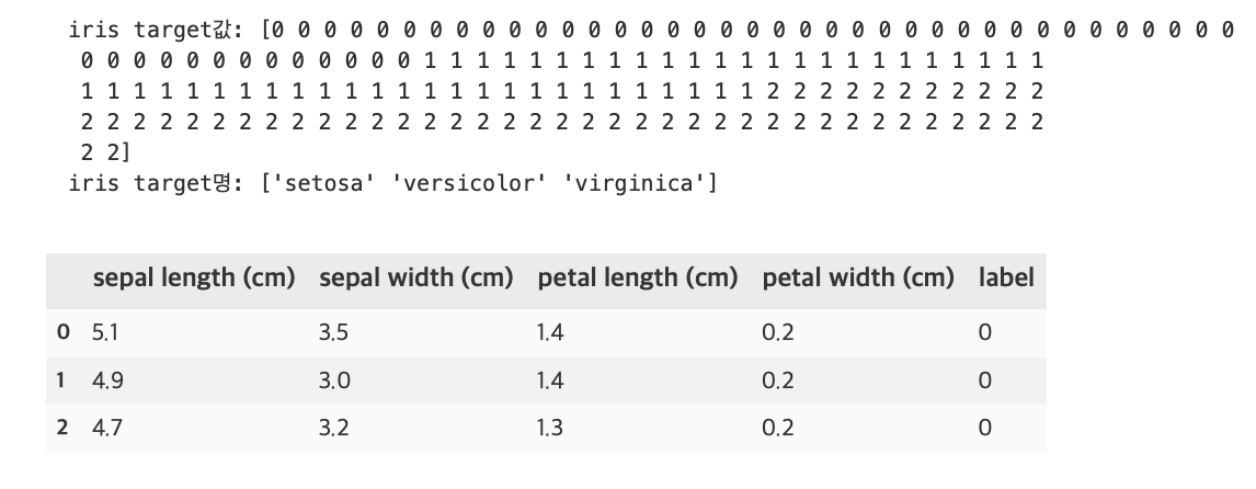

특징으로는 sepal length, sepal width, petal length, petal width가 있고, 레이블은 0, 1, 2 세가지 값이 있다. 0이 setosa 품종, 1이 versicolor 품종, 2가 virginica 품종이다.

X_train, X_test, y_train, y_test = train_test_split(iris_data, iris_label, test_size=0.2, random_state=11)

random_state를 지정하지 않으면 수행할 때마다 다른 학습/테스트 용 데이터를 만들 수 있으므로 임의의 수를 부여함(어떤 숫자여도 상관 없음)
test_size=0.2는 전체 데이터 세트 중 테스트 데이터 세트의 비율이다.

• X_train: 학습용 피처 데이터 세트
• X_test: 테스트용 피처 데이터 세트
• y_train: 학습용 레이블 데이터 세트
• y_test: 테스트용 레이블 데이터 세트

dt_clf = DecisionTreeClassifier(random_state=11)
dt_clf.fit(X_train, y_train)

DecisionTreeClassifier(random_state=11)
fit()메서드에 학습용 피처 데이터 속성과 결정 값 데이터 세트를 입력해 호출하면 학습을 수행한다.

pred = dt_clf.predict(X_test)

predict()메서드에 테스트용 피처 데이터 세트를 입력해 호출하면 학습된 모델 기반에서 테스트 데이터 세트에 대한 예측값을 반환한다.

from sklearn.metrics import accuracy_score
print(f'예측 정확도: {round(accuracy_score(y_test, pred),4)}')

예측 정확도: 0.9333
accuracy_score()의 첫 번째 파라미터로 실제 레이블 데이터 세트, 두 번째 파라미터로 예측 레이블 데이터 세트를 입력하면 된다.

사이킷런의 기반 프레임워크 익히기

사이킷런은 매우 많은 유형의 Classifier와 Regressor 클래스를 제공하고, 이들을 합쳐서 Estimator 클래스라고 부른다.

Estimator

학습: fit()
예측: predict()

1. Classifier(분류)
   • DecisionTreeClassifier
   • RandomForestClassifier
   • GradientBoostingClassifier
   • GaussianNB
   • SVC
2. Regressor(회귀)
   • LinearRegression
   • Ridge
   • Lasso
   • RandomForestRegressor
   • GradientBoostingRegressor

사이킷런에 내장된 데이터 세트는 일반적으로 딕셔너리 형태로 되어 있다.
키는 보통 data, target, target_names, feature_names, DESCR로 구성되어 있다.

• data: 피처의 데이터 세트를 가리킨다.
• target: 분류 시 레이블 값, 회귀 시 숫자 결과값 데이터 세트이다.
• target_names: 개별 레이블의 이름을 나타낸다.
• feature_names: 피처의 이름을 나타낸다.
• DESCR: 데이터 세트에 대한 설명과 각 피처의 설명을 나타낸다.

data, target은 넘파이 배열(ndarray) 타입이며, target_names, feature_names는 넘파이 배열 또는 파이썬 리스트 타입이고 DESCR은 스트링 타입이다.

iris_data = load_iris()
print(type(iris_data))

<class 'sklearn.utils.Bunch'>
Bunch 클래스는 파이썬 딕셔너리 자료형과 유사하므로 데이터 세트의 key 값을 확인할 수 있다.

keys = iris_data.keys()
print(f'붓꽃 데이터 세트의 키들: {keys}')

붓꽃 데이터 세트의 키들: dict_keys(['data', 'target', 'frame', 'target_names', 'DESCR', 'feature_names', 'filename'])

학습/테스트 데이터 세트 분리 - train_test_split()

전체 데이터를 학습 데이터와 테스트 데이터로 분리하는 작업은 꼭 필요하다. 그럼 만약 학습 데이터로만 학습하고 예측하면 어떤 문제가 발생하는지 알아보자.

iris = load_iris()
dt_clf = DecisionTreeClassifier()
train_data = iris.data
train_label = iris.target
dt_clf.fit(train_data, train_label)

pred = dt_clf.predict(train_data)
print(f'예측 정확도: {accuracy_score(train_label, pred)}')

예측 정확도: 1.0
정확도가 100%라 아주 정확하게 예측한 것 같지만 사실 이미 학습한 데이터 세트를 기반으로 예측했기에 이러한 결과가 나온다. 예측을 하는 데이터 세트는 학습을 수행한 학습용 데이터 세트가 아닌 테스트 데이터 세트를 이용해야한다.

train_test_split()의 파라미터로 피처 데이터 세트, 레이블 데이터 세트를 받고 선택적으로 아래 파라미터들을 받는다.

• test_size: 전체 데이터에서 테스트 데이터 세트 크기를 얼마로 샘플링할 것인가를 결정한다. 디폴트는 0.25(25%)
• train_size: 전체 데이터에서 학습용 데이터 세트 크기를 얼마로 샘플링할 것인가를 결정한다. 일반적으로 test_size 파라미터를 사용하기에 잘 사용하지 않는다.
• shuffle: 데이터를 분리하기 전에 데이터를 미리 섞을지 결정한다. 디폴트는 True, 데이터를 분산시켜서 좀 더 효율적인 학습 및 테스트 데이터 세트를 만드는데 사용된다.
• random_state: train_test_spit()은 호출 시 무작위로 데이터를 분리하므로 random_state를 지정하지 않으면 수행할때마다 다른 학습/테스트용 데이터를 생성한다.
• train_test_split()의 반환값은 튜플 형태이고, 학습용 데이터의 피처 데이터 세트, 테스트용 데이테의 피처 데이터 세트, 학습용 데이터의 레이블 데이터 세트, 테스트용 데이터의 레이블 데이터 세트 순으로 반환된다.

# 앞의 예제와 다르게 테스트 데이터 세트를 전체의 30%로, random_state=121로 설정
dt_clf = DecisionTreeClassifier()
iris_data = load_iris()

X_train, X_test, y_train, y_test = train_test_split(iris_data.data, iris_data.target, test_size=0.3, random_state=121)

dt_clf.fit(X_train, y_train)
pred = dt_clf.predict(X_test)
print(f'예측 정확도: {round(accuracy_score(y_test, pred), 4)}')

예측 정확도: 0.9556

교차검증 - K Fold

가장 보편적으로 사용되는 교차 검증 기법으로 먼저 k개의 데이터 폴드 세트를 만들어서 k번만큼 각 폴드 세트에 학습과 검증 평가를 반복적으로 수행하는 방법
예를 들어 4폴드 교차 검증을 수행하면 4개 데이터를 각각 한번씩 검증 데이터로 설정하고 나머지 3개를 학습 데이터로 설정하여 학습 및 평가 후 4개의 결과를 평균해서 K 폴드 평가 결과로 반영한다.

from sklearn.model_selection import KFold

iris = load_iris()
features = iris.data
label = iris.target
dt_clf = DecisionTreeClassifier(random_state=156)

kfold = KFold(n_splits=5)
cv_accuracy = []
print(f'붓꽃 데이터 세트 크기: {features.shape[0]}')

붓꽃 데이터 세트 크기: 150

import numpy as np

n_iter = 0

for train_index, test_index in kfold.split(features):
    X_train, X_test = features[train_index], features[test_index]
    y_train, y_test = label[train_index], label[test_index]
    
    # 학습 및 예측
    dt_clf.fit(X_train, y_train)
    pred = dt_clf.predict(X_test)
    n_iter += 1
    
    # 반복할 때마다 정확도 측정
    accuracy = np.round(accuracy_score(y_test, pred), 4)
    train_size = X_train.shape[0]
    test_size = X_test.shape[0]
    print('\n#{0} 교차 검증 정확도: {1}, 학습 데이터 크기: {2}, 검증 데이터 크기: {3}'.format(n_iter, accuracy, train_size,test_size))
    print('#{0} 검증 세트 인덱스: {1}'.format(n_iter, test_index))
    cv_accuracy.append(accuracy)
    
# 개별 iter별 정확도로 평균 정확도 계산
print('\n## 평균 검증 정확도:', np.mean(cv_accuracy))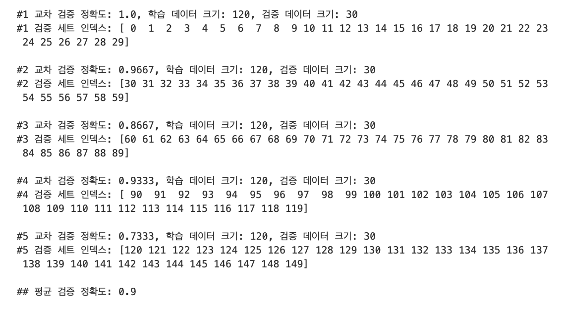

Stratified K 폴드

Stratified K 폴드는 불균형한 분포도를 가진 레이블 데이터 집합을 위한 K 폴드 방식이다. 불균형한 분포도를 가진 레이블 데이터 집합은 특정 레이블 값이 특이하게 많거나 매우 적어서 값의 분포가 한쪽으로 치우치는 것을 말한다.

iris = load_iris()
iris_df = pd.DataFrame(data=iris.data, columns=iris.feature_names)
iris_df['label'] = iris.target
iris_df['label'].value_counts()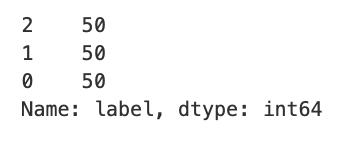

레이블 값은 0, 1, 2 값 모두 50개로 동일한데, 이슈가 발생하는 현상을 도출하기 위해 3개의 폴드 세트를 KFold로 생성하고, 각 교차 검증 시마다 생성되는 학습/검증 레이블 데이터 값의 분포도를 확인해보자.

kfold = KFold(n_splits=3)
n_iter = 0
for train_index, test_index in kfold.split(iris_df):
    n_iter += 1
    label_train = iris_df['label'].iloc[train_index]
    label_test = iris_df['label'].iloc[test_index]
    print(f'## 교차 검증: {n_iter}')
    print(f'학습 레이블 데이터 분포:\n{label_train.value_counts()}')
    print(f'검증 레이블 데이터 분포:\n{label_test.value_counts()}')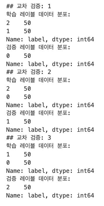

첫 번째 교차 검증에서 학습 레이블의 1, 2 값이 각각 50개가 추출되었고, 검증 레이블의 0 값이 50개가 추출되었다. 학습 레이블이 1, 2밖에 없기에 0의 경우는 전혀 학습할 수 없고, 반대로 검증 레이블은 0밖에 없으므로 학습 모델은 절대 0을 예측하지 못한다. 이러한 유형으로 교차 검증 데이터 세트를 분할하면 검증 예측 정확도는 0이 될 수밖에 없다.
우리는 StratifiedKFold를 통해 이 문제를 해결해 볼 수 있다.

from sklearn.model_selection import StratifiedKFold

skf = StratifiedKFold(n_splits=3)
n_iter = 0

for train_index, test_index in skf.split(iris_df, iris_df['label']):
    n_iter += 1
    label_train = iris_df['label'].iloc[train_index]
    label_test = iris_df['label'].iloc[test_index]
    print(f'## 교차 검증: {n_iter}')
    print(f'학습 레이블 데이터 분포:\n{label_train.value_counts()}')
    print(f'검증 레이블 데이터 분포:\n{label_test.value_counts()}')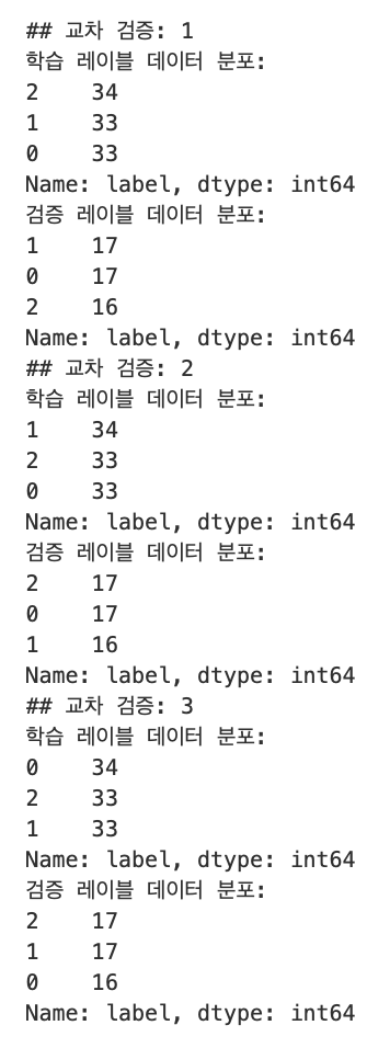

첫 번째 교차 검증에서 학습 레이블은 0, 1, 2 값이 각각 33-34개로, 레이블별로 동일하게 할당되었고, 검증 레이블도 0, 1, 2 값이 각각 16-17개로 동일하게 할당되었으므로 레이블 값 0, 1, 2를 모두 학습할 수 있고 검증을 수행할 수 있다.
이번엔 붓꽃 데이터를 교차 검증해보자.

dt_clf = DecisionTreeClassifier(random_state=156)
    
skfold = StratifiedKFold(n_splits=3)
n_iter = 0
cv_accuracy = []

# StratifiedKFold의 split() 호출시 반드시 레이블 데이터 세트도 추가 입력 필요
for train_index, test_index in skfold.split(features, label):
    X_train, X_test = features[train_index], features[test_index]
    y_train, y_test = label[train_index], label[test_index]
    
    dt_clf.fit(X_train, y_train)
    pred = dt_clf.predict(X_test)
    
    n_iter += 1
    accuracy = np.round(accuracy_score(y_test, pred), 4)
    train_size = X_train.shape[0]
    test_size = X_test.shape[0]
    print('\n#{0} 교차 검증 정확도: {1}, 학습 데이터 크기: {2}, 검증 데이터 크기: {3}'.format(n_iter, accuracy, train_size, test_size))
    print('#{0} 검증 세트 인덱스: {1}'.format(n_iter, test_index))
    cv_accuracy.append(accuracy)

# 교차 검증별 정확도 및 평균 정확도 계산
print(f'\n## 교차 검증별 정확도: {np.round(cv_accuracy, 4)}')
print(f'## 평균 검증 정확도: {np.mean(cv_accuracy)}')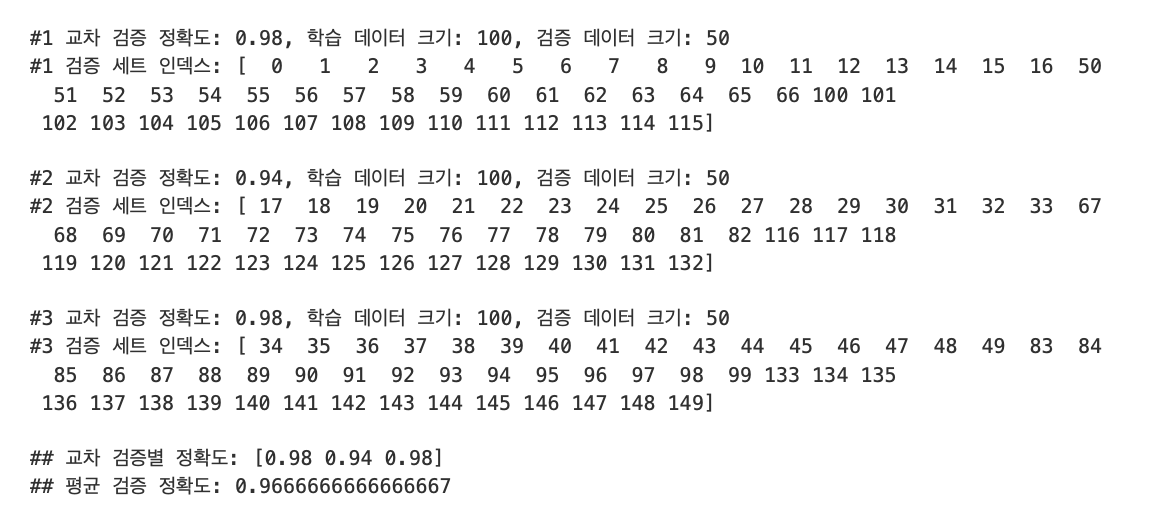

교차 검증을 편하게 하기 - cross_val_score()

cross_val_score(estimator, X, y=None, scoring=None, cv=None, n_jobs=1, verbose=0, fit_params=None, pre_dispatch='2*n_jobs')
이 중에서 estimator, X, y, scoring, cv가 주요 파라미터이다.

• estimator: 분류 알고리즘 클래스 Classifier 또는 회귀 알고리즘 클래스 Regressor
• X: 피처 데이터 세트
• y: 레이블 데이터 세트
• scoring: 예측 성능 평가 지표
• cv: 교차 검증 폴드 수

from sklearn.model_selection import cross_val_score, cross_validate

iris_data = load_iris()
dt_clf = DecisionTreeClassifier(random_state=156)

data = iris_data.data
label = iris_data.target

# 성능 지표는 정확도(Accuracy), 교차 검증 세트는 3개
scores = cross_val_score(dt_clf, data, label, scoring='accuracy', cv=3)
print(f'교차 검증별 정확도: {np.round(scores, 4)}')
print(f'평균 검증 정확도: {np.round(np.mean(scores), 4)}')

교차 검증별 정확도: [0.98 0.94 0.98]
평균 검증 정확도: 0.9667
cross_val_score()가 내부적으로 StratifiedKFold를 이용해서 앞서 수행한 예제의 결과와 정확도가 동일하다.

교차 검증과 최적 하이퍼 파라미터 튜닝 한번에 하기 - GridSearchCV

GridSearchCV 클래스의 생성자로 들어가는 주요 파라미터

• estimator: classifier, regressor, pipeline이 사용됨
• param_grid: key + 리스트 값을 가지는 딕셔너리가 주어짐.
• scoring: 예측 성능을 측정할 평가 방법을 지정. 일반적으로 'accuracy'로 지정
• cv: 교차 검증을 위해 분할되는 학습/테스트 세트의 갯수
• refit: 디폴트는 True, 가장 최적의 하이퍼 파라미터를 찾은 뒤 입력된 estimator 객체를 해당 하이퍼 파라미터로 재학습함.

아래 예제는 붓꽃 데이터를 train_test_split()을 이용해 학습 데이터와 테스트 데이터로 분리한 후, 학습 데이터에서 GridSearchCV를 이용해 최적 하이퍼 파라미터를 추출하고, 결정 트리 알고리즘의 중요 하이퍼 파라미터인 max_depth와 min_samples_split의 값을 변화시키면서 최적화를 진행하려 한다.

from sklearn.model_selection import GridSearchCV

iris_data = load_iris()
X_train, X_test, y_train, y_test = train_test_split(iris_data.data, iris_data.target, test_size=0.2, random_state=121)
dtree = DecisionTreeClassifier()

parameters = {'max_depth': [1, 2, 3],
             'min_samples_split': [2, 3]
             }

grid_dtree = GridSearchCV(dtree, param_grid=parameters, cv=3, refit=True)
grid_dtree.fit(X_train, y_train)

scores_df = pd.DataFrame(grid_dtree.cv_results_)
scores_df[['params', 'mean_test_score', 'rank_test_score', 'split0_test_score', 'split1_test_score', 'split2_test_score']]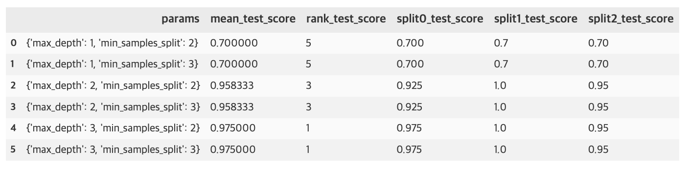

print(f'GridSearchCV 최적 파라미터: {grid_dtree.best_params_}')
print('GridSearchCV 최고 정확도: {0:.4f}'.format(grid_dtree.best_score_))

estimator = grid_dtree.best_estimator_

pred = estimator.predict(X_test)
print('테스트 데이터 세트 정확도: {0:.4f}'.format(accuracy_score(y_test, pred)))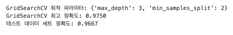

Source: 파이썬 머신러닝 완벽 가이드 / 위키북스