주제 선정

첫 프로젝트 이후로는 머신러닝, 딥러닝 원리와 이 분야의 Python 라이브러리 활용법을 배웠다. 머신러닝 분야를 대표하는 라이브러리 scikit-learn, 딥러닝 분야를 대표하는 라이브러리 tensorflow를 배우고 익힌 뒤 이를 활용하는 조별 프로젝트가 진행되었다.

우리 조는 음성 데이터를 통해 목소리 성별을 구별하는 프로젝트를 진행하기로 했다. Kaggle에서 발견한 음성 데이터 자료 "Gender Recognition by Voice"를 기반으로 머신러닝 및 딥러닝 모델을 만든 뒤, 우리가 직접 만든 음성 데이터를 학습 완료된 모델에 적용시켜 제대로 작동하는지 확인하는 것을 목표로 삼았다.

데이터 수집 및 전처리

Kaggle에는 해당 데이터를 활용한 코드 예시가 데이터와 함께 업로드되어 있었다. 우리는 머신러닝 모델을 만들 때는 "Voice classification from numerical features", 딥러닝 모델을 만들 때는 "Voice Recognition using Tensorflow" 포스팅의 코드를 참고하였다.

원본 데이터가 굉장히 잘 정리되어 있었다. 원본 데이터는 여러 대학교에서 수집한 목소리 자료 3168개를 요소별로 분석한 뒤 모아놓은 자료로, 결측치가 없었다. 남녀 목소리의 갯수 역시 동일했다. 인간 목소리의 주파수는 특성상 범위가 정해져 있었기 때문에 전처리에서 문제를 겪을 여지가 적었다.

중요 feature 판별

원본 데이터를 voice_df 변수로 불러오고 성별을 각각 "female"=0, "male"=1로 변환한 뒤, 성별에 따라 각 변수가 어느 정도의 차이를 보이는지 시각화하여 확인해 보았다.

plt.subplots(4,5,figsize=(25,20))
for k in range(1,21):
    plt.subplot(4,5,k)
    plt.title(voice_df.columns[k-1])
    sns.kdeplot(voice_df.loc[voice_df['label'] == 0, voice_df.columns[k-1]], color= 'green', label='F')
    sns.kdeplot(voice_df.loc[voice_df['label'] == 1, voice_df.columns[k-1]], color= 'red', label='M')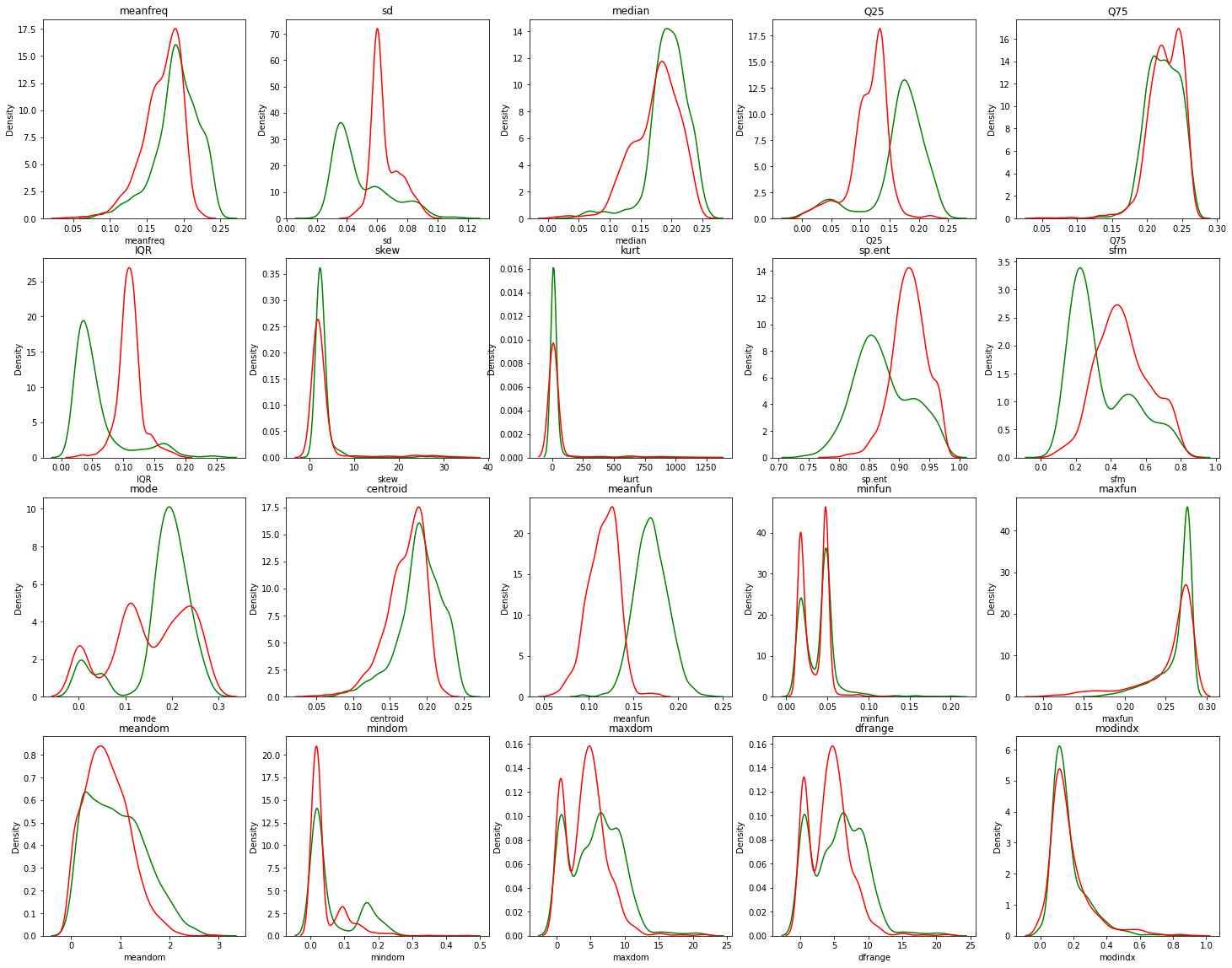

그 결과 성별 판정에 가장 영향을 많이 미치는 독립변수는 총 3가지라고 보았다.

• 분위수의 범위(IQR) : 상위75% 지점의 값과 하위 25% 지점의 값에 대한 차이
• 1분위값(Q25) : 하위 25%에 대한 값
• 주파수의 평균(meanfun) : 목소리 높이의 평균

따라서 우리는 위 3가지 feature를 변수로 삼아 머신러닝 모델을 설계해 보았다.

머신러닝 모델 활용 (sklearn)

우리는 머신러닝 모델로 LogisticRegression, KNeighborsClassifier, Support Vector Machine, RandomForestClassifier, DecisionClassifier 총 6개를 만든 뒤 정확도를 비교하여 그중 가장 나은 모델을 최종 테스트용으로 결정하였다.

데이터 분리, 모델 선정 (변수 TOP 3)

우선 데이터에서 feature 3개를 분리하고 train_test_split 과정을 거쳤다.

features = voice_df.loc[:,['Q25', 'meanfun', 'IQR']]    # 가장 상관관계가 높은 변수만 포함하기
target = voice_df.iloc[:,-1]
features.shape, target.shape
type(features), type(target)
--> (pandas.core.frame.DataFrame, pandas.core.series.Series)

X_train, X_test, y_train, y_test = train_test_split(features, target, test_size=0.2, random_state=121)
X_train.shape, y_train.shape
--> ((2534, 3), (2534,))

이후 여러 가지 모델을 만들어 가장 정확도 높은 모델을 골라내기로 했다.

regressionModel = LogisticRegression()  
regressionModel.fit(X_train,y_train)
regressionModel.score(X_train,y_train)

KNNModel = KNeighborsClassifier(n_neighbors=3) 
KNNModel.fit(X_train,y_train)
KNNModel.score(X_train,y_train)

svmRbfModel=sklearn.svm.SVC(kernel='rbf',C=10) 
svmRbfModel.fit(X_train,y_train)
svmRbfModel.score(X_train,y_train)

svmPolyModel=sklearn.svm.SVC(kernel='poly',C=10000)
#다항식을 이용할 경우 poly
svmPolyModel.fit(X_train,y_train)
svmPolyModel.score(X_train,y_train)

randomFModel = RandomForestClassifier(max_depth=3,min_samples_split=2) 
randomFModel.fit(X_train, y_train)
randomFModel.score(X_train,y_train)

dTreeModel = DecisionTreeClassifier(max_depth=3,min_samples_split=2) 
randomFModel.fit(X_train, y_train)
dTreeModel.fit(X_train, y_train)
dTreeModel.score(X_train,y_train)

해당 모델들의 정확도를 표와 그래프로 나타내어 어느 모델을 활용할 지 결정하였다.

trainScores = [regressionModel.score(X_train, y_train), KNNModel.score(X_train, y_train),svmRbfModel.score(X_train, y_train),svmPolyModel.score(X_train, y_train), randomFModel.score(X_train,y_train), dTreeModel.score(X_train,y_train)]
testScores = [regressionModel.score(X_test, y_test), KNNModel.score(X_test, y_test), svmRbfModel.score(X_test, y_test),svmPolyModel.score(X_test, y_test), randomFModel.score(X_test,y_test), dTreeModel.score(X_test,y_test)]
indices = ['Logistic Regression', 'KNN', 'SVM-RBF','SVM-Poly', 'RandomForest', 'DecisionTree']
scores = pd.DataFrame({'Training Score': trainScores,'Testing Score': testScores}, index=indices) #모델별로 train 정확도와 test정확도의 결과값들을 비교해봤습니다.

scores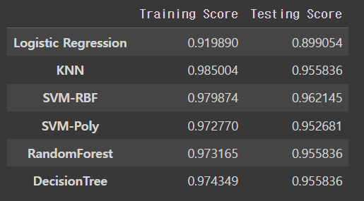

plot = scores.plot.bar(figsize=(16, 8), rot=0)
plt.title('Training and Testing Scores')
plt.show()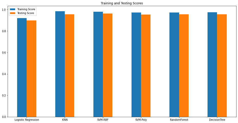

우리는 Training Score, Testing Score가 가장 높은 DecisionTree 모델을 이후 검증에 이용하기로 했다.

실전 테스트 (변수 TOP 3)

우리는 모델을 만든 뒤 테스트할 데이터로 총 6개의 목소리 샘플을 만들었다. 목소리 샘플은 각각 카운터테너 목소리, 일반인 남성 고음 목소리, 일반인 남성 저음 목소리, 배우 김혜수 목소리, 일반인 여성 목소리, 짱구 목소리에서 따왔다. 일반적인 남녀 목소리뿐만 아니라, 남성이 여성, 여성이 남성 음역대를 내는 데이터를 수집하여 모델을 엄밀하게 검증하려고 했다.

해당 목소리를 원본 데이터와 동일한 형태로 변환하기 위하여 Kaggle 데이터 업로더가 제공한 R 코드를 활용하였다. 변환 결과를 test_df1 변수에 저장하였다.

test_df1 = test_df.copy()
test_df1.drop(['meanfreq','maxdom','sd','median','Q75','skew','kurt','sp.ent','sfm','mode','centroid','minfun','maxfun','meandom','mindom','dfrange','modindx'], axis = 1,inplace=True)
pred = KNNModel.predict(test_df1.drop(['label'],axis=1))
pred
--> array([1, 1, 1, 1, 1, 1])

모델이 기존에 보여준 높은 정확도와는 달리, 새 데이터에 대한 예측력은 낮았다. 영향력 높은 변수만을 뽑아 모델로 검증하는 것이 결코 좋은 예측력을 보장하지 않는다는 것을 잘 알게 되었다. 따라서 아래에서는 전체 feature를 통해 모델을 만들고 검증하기로 했다.

전체 변수

features = voice_df.iloc[:, :-1]   # 모든 feature 변수 넣기
target = voice_df.iloc[:,-1]
features.shape, target.shape
type(features), type(target)
--> (pandas.core.frame.DataFrame, pandas.core.series.Series)

X_train, X_test, y_train, y_test = train_test_split(features, target, test_size=0.2, random_state=121)
X_train.shape, y_train.shape
--> ((2534, 20), (2534,))

이후 위와 동일한 코드로 동일한 모델을 설계 및 학습 진행하였다.

trainScores = [regressionModel.score(X_train, y_train), KNNModel.score(X_train, y_train),svmRbfModel.score(X_train, y_train),svmPolyModel.score(X_train, y_train), randomFModel.score(X_train,y_train), dTreeModel.score(X_train,y_train)]
testScores = [regressionModel.score(X_test, y_test), KNNModel.score(X_test, y_test), svmRbfModel.score(X_test, y_test),svmPolyModel.score(X_test, y_test), randomFModel.score(X_test,y_test), dTreeModel.score(X_test,y_test)]
indices = ['Logistic Regression', 'KNN', 'SVM-RBF','SVM-Poly', 'RandomForest', 'DecisionTree']
scores = pd.DataFrame({'Training Score': trainScores,'Testing Score': testScores}, index=indices) #모델별로 train 정확도와 test정확도의 결과값들을 비교해봤습니다.

scores

plot = scores.plot.bar(figsize=(16, 8), rot=0)
plt.title('Training and Testing Scores')
plt.show()  #모델별로 train 정확도와 test의 정확도의 결과값들을 그래프로 나타내봤습니다.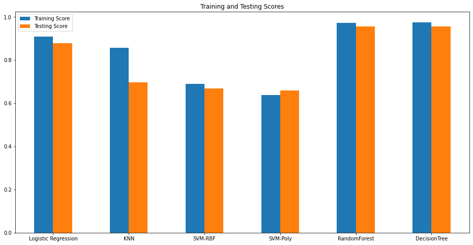

모델 만들기에 반영된 feature의 갯수가 늘어났지만, 가장 정확도가 높은 모델은 DecisionTree로 동일하였다.

test_df2 = test_df.copy()

# object 형태인 데이터를 숫자로 바꿔주기 - female => 0, male => 1
test_df2.replace(to_replace="female", value=0, inplace=True)
test_df2.replace(to_replace="male", value=1, inplace=True)
test_df2.label.unique() # df의 label명을 여성은 0, 남성은 1로 변환했음.

pred = dTreeModel.predict(test_df2.drop(['label'],axis=1))
pred
--> array([1, 0, 1, 0, 0, 0])

accuracy_score((test_df2.label), pred)
--> 0.8333333333333334

영향력이 낮은 feature까지 모두 학습시킨 모델이 실전 데이터를 판별하는 데에는 훨씬 높은 성능을 냈다.

딥러닝 모델 활용 (tensorflow)

머신러닝 모델을 만들어 어느 정도 검증력을 확보해 본 뒤, 딥러닝으로 더 높은 성능을 가진 모델을 만들 수 있을지 궁금해졌다.

Sigmoid

# relu -> sigmoid & dropout 세줄에 한번 추가
model = Sequential()
model.add(Dense(256, input_shape=(20,)))
model.add(Dense(128, activation="relu"))
model.add(Dense(64, activation="relu"))
model.add(Dropout(0.3))
model.add(Dense(32, activation="relu"))
model.add(Dense(16, activation="relu"))
model.add(Dense(1, activation="sigmoid"))

# sigmoid와 binary crossentropy를 이용한 이유는 male/female 2개의 바이너리이기 때문에

model.compile(loss="binary_crossentropy", metrics=["accuracy"], optimizer=tf.keras.optimizers.Adam(lr=0.001))

model.fit(X_train, y_train, epochs=100,
          batch_size=64, validation_split=0.25,
          callbacks=[EarlyStopping(monitor='val_loss', patience=10)])
          
# evaluating the model using the testing set
print(f"Evaluating the model using {len(X_test)} samples...")
loss, accuracy = model.evaluate(X_test,y_test, verbose=0)
print(f"Loss: {loss:.4f}")
print(f"Accuracy: {accuracy*100:.2f}%")
--> Evaluating the model using 634 samples...
Loss: 0.1439
Accuracy: 94.16%

실전 테스트 (Sigmoid)

test_df2.label
--> 0    1
1    1
2    1
3    0
4    0
5    0
Name: label, dtype: int64

pred = model.predict(test_df2.drop(['label'],axis=1))
# 0,0,1,0,0,0      # 1,1,1,0,0,0
--> array([[3.5717976e-01],
       [1.6104305e-01],
       [9.9165469e-01],
       [3.8860559e-02],
       [1.4352798e-04],
       [2.2471845e-03]], dtype=float32)
       
# 테스트
print(f"Evaluating the model using {len(X_test)} samples...")
loss, accuracy = model.evaluate(test_df2.drop(['label'],axis=1), test_df2.label, verbose=0)
print(f"Loss: {loss:.4f}")
print(f"Accuracy: {accuracy*100:.2f}%")
--> Evaluating the model using 634 samples...
Loss: 0.4843
Accuracy: 66.67%

딥러닝 모델의 정확도는 결코 높지 않았다. 하지만 마지막 activation 함수를 sigmoid 함수에서 softmax 함수로 바꾸면 정확도가 높아질 수도 있을 것 같았다.

Softmax

# relu -> softmax & dropout
model = Sequential()
model.add(Dense(256, input_shape=(20,)))
model.add(Dense(128, activation="relu"))
model.add(Dense(64, activation="relu"))
model.add(Dropout(0.3))
model.add(Dense(32, activation="relu"))
model.add(Dense(16, activation="relu"))
model.add(Dense(2, activation="softmax"))

model.compile(loss="sparse_categorical_crossentropy", metrics=["accuracy"], optimizer="adam")

model.fit(X_train, y_train, epochs=100,
          batch_size=64,
          callbacks=[EarlyStopping(monitor='val_loss', patience=10)])
          
# 평가하는 세트
print(f"Evaluating the model using {len(X_test)} samples...")
loss, accuracy = model.evaluate(X_test,y_test, verbose=0)
print(f"Loss: {loss:.4f}")
print(f"Accuracy: {accuracy*100:.2f}%")
--> Evaluating the model using 634 samples...
Loss: 0.1686
Accuracy: 94.01%

실전 테스트 (Softmax)

pred = model.predict(test_df2.drop(['label'],axis=1))
pred
# 0,0,1,0,0,0
--> array([[7.6749623e-01, 2.3250371e-01],
       [8.5192752e-01, 1.4807250e-01],
       [2.6076129e-03, 9.9739242e-01],
       [5.7367176e-01, 4.2632824e-01],
       [9.9943155e-01, 5.6848244e-04],
       [9.8048556e-01, 1.9514462e-02]], dtype=float32)
 
# 평가하는 세트
print(f"Evaluating the model using {len(X_test)} samples...")
loss, accuracy = model.evaluate(test_df2.drop(['label'],axis=1), test_df2.label, verbose=0)
print(f"Loss: {loss:.4f}")
print(f"Accuracy: {accuracy*100:.2f}%")
--> Evaluating the model using 634 samples...
Loss: 0.6579
Accuracy: 66.67%

activation 함수를 바꿨지만 실전 데이터에 대한 예측력은 여전히 낮았다. 딥러닝 기법은 학습 대상인 데이터의 수가 많아야 좋은 예측력을 낼 수 있는데, 원본 데이터의 갯수(3168개)는 딥러닝으로 좋은 예측력을 내기에 너무 적은 수였던 것 같다.

결론

프로젝트 중 활용한 여러 모델 중, 전체 feature를 학습한 DecisionTree 모델이 가장 높은 예측력을 냈다.

영향력이 낮은 feature까지 전부 포함하여 학습시킨 모델이 영향력 높은 feature만 취사선택한 모델보다 예측력이 좋았고, 데이터 수가 비교적 적은 경우 딥러닝보다 머신러닝 모델의 예측력이 좋을 수 있다는 것을 알게 되었다. 또한 많은 경우 머신러닝 모델을 여러 개 묶어 검증하는 모델이 높은 예측력을 보이곤 했지만, 우리 프로젝트에서는 모델 1개만을 활용하는 경우와 모델 여러 개를 묶은 경우가 비슷한 예측력을 보였다.

나중에 발명된 모델이 이전에 발명된 모델보다 무조건 좋은 성능을 내는 것이 아니며, 데이터 특성, 목적, 분량 등을 고려하여 상황에 따라 다양한 모델을 취사 선택하여 활용하는 것이 좋을 것 같았다.

의욕 넘치고 똑똑한 조원 네 분과 함께한 덕분에 좋은 성과를 낼 수 있었다. 짧은 시간 안에 많은 작업을 수행하며 얻어가는 것도 많았고, 집중해서 작업한 만큼 즐거움도 더 많이 느낄 수 있었다. 함께해주신 분들께 정말 감사드린다.