260206 [ Day 27 ] - ML, DL (4)

시작하며

오늘로 통계학 내용은 마무리가 되었다. 정말 어렵고 복잡한 내용이 많았지만 묘하게 재미가 있어서 이후에 강사님께서 추천해주신 책을 구매해서 통계학도 공부해보고 싶다.

영향점

• 스튜던트 잔차 : y중심
• 레버리지 : x중심
• 쿡의 거리 : 쿡의 거리가 4/n(행 개수)보다 큰 관측값을 영향점으로 의심 할 수 있음

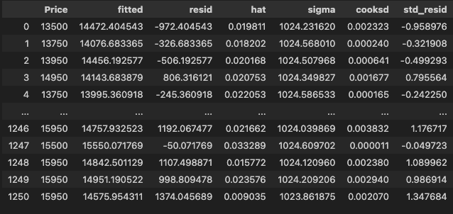
aug = hds.stat.augment(model=model)

• fitted : 추정값
• resid : 잔차
• hat : 레버리지
• sigma : 해당 관측값 제거한 후 표준편차 추정값
• cooksd : 쿡의 거리
• std_resid : 표준화 잔차

sigma 가 작을수록, cooksd 가 클수록 해당 관측값을 이상치로 판단

• 이상치 값 인덱스 추출

out_index = aug.loc[aug['cooksd'].gt(4 / X.shape[0])].index

• 영향점 시각화

plt.figure(figsize=(4, 4))
sns.regplot(
    data=df, x='Age', y='Price', ci=None,
    scatter_kws={'color': '0.8', 's': 10, 'ec': '0.8'},
    line_kws={'color': 'red', 'lw': 1.5}
)
sns.scatterplot(
    data=df.loc[out_index, :], x='Age', y='Price',
    fc='red', ec='red', s=20, label='Outlier'
)
plt.legend()

plt.show()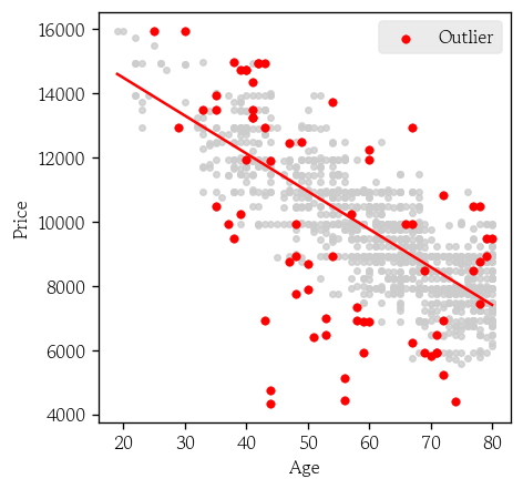

• 영향점 제거

X = X.drop(index=out_index)
y = y.drop(index=out_index)

• 영향치 제거한 모형

model = hds.stat.ols(X=X, y=y)
model.summary()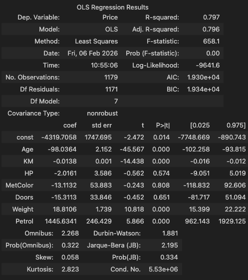

stats.shapiro(model.resid)
# ShapiroResult(statistic=np.float64(0.9987108551069022), pvalue=np.float64(0.5564148139317799))

hds.stat.breushpagan(model=model)
#   Statistic	P-Value	  F-Value	  F P-Value
# 0	14.124654	0.049008	2.028417	0.048685

다중공선성

변수 ⬆️ → $R^2$ ⬆️ → MSE ⬇️
변수 ⬇️ → $R^2$ ⬇️ → MSE ⬆️

• 입력변수 간 강한 상관관계가 있으면 다중공선성문제가 발생
  • 강한 상관관계를 갖는 입력변수들은 목표변수에 대한 설명력을 나누어 가져 신뢰할 수 없게 됨
  • 회귀계수의 표준오차가 증가 → 회귀계수의 설명력 낮아짐

분산팽창지수(VIF)

• 다중 선형 회귀 모형에서 입력변수가 다른 입력변수에 종속 여부를 판단할 때 계산
• 각 입력변수를 목표변수로 설정하여 나머지 변수들로 모형 적합
  • $VIF_j = \frac{1}{1 - R^2_j}$
  • 결정계수 0.8 → VIF 5
  • 결정계수 0.9 → VIF 10
• VIF가 5 이상이면 다중공선성 문제가 있을 가능성 있음
  • 10 이상이면 매우 심각한 문제가 있다고 판단

다중공선성 확인

hds.stat.vif(model=model)
#   Age	      KM	      HP	      MetColor	Doors	    Weight	  Petrol
# 0	1.335567	1.609369	3.123682	1.015065	1.633648	4.762933	6.615611

• 다중공선성 문제 해결

X = X.drop(columns='Petrol')
model = hds.stat.ols(X=X, y=y)
hds.stat.vif(model=model)
#   Age	      KM	      HP	    MetColor	Doors	    Weight
# 0	1.333597	1.498871	1.13305	1.013634	1.279331	1.457494

변수선택법

• 입력변수의 모든 경우의 수를 고려하여 성능이 우수한 최종 회귀 모형을 선택
  • 입력변수가 p개일 때 → $2^p$ 개의 후보 모형을 생성해야 함
• 전진선택법, 후진소거법, 단계적방법으로 적합
  • AIC가 가장 작은 모형을 선택

AIC

• 모형의 적합도와 복잡도를 고려한 평가 지표
  • 모형의 적합도 : 최대 가능도
  • 복잡도 : 모형에 사용된 변수의 개수
  • 오차항이 정규분포를 따르면, 최대 가능도는 잔차제곱합으로 표현
    • $AIC = 2p - 2\ln(L)$
• AIC 값이 작을수록 좋은 모형이라고 판단
  • 좋은 변수 → AIC ⬇️
  • 나쁜 변수 → AIC ⬆️

전진선택법

• 입력변수를 하나씩 추가하면서 최적의 회귀 모형을 탐색
  • Null 모형에서 입력변수를 하나씩 추가 → 그 중에서 AIC가 가장 작은 후보 모형을 선택
    
  • 이전 단계 회귀 모형보다 AIC가 작은 후보 모형이 없으면 중단
  • 최대 $\frac{p(p + 1)}{2}$개 후보 모형을 적합
  • 한 번 선택한 입력변수를 제거할 수 없음

후진소거법

• 입력변수를 하나씩 제거하면서 최적의 회귀 모형을 탐색
  • Full 모형에서 입력변수를 하나씩 제거 → 그 중에서 AIC가 가장 작은 후보 모형을 선택
    
  • 최대 $\frac{p(p + 1)}{2}$개 후보 모형을 적합
  • 한 번 제거한 입력변수를 추가할 수 없음

단계적방법

• 전진선택법과 후진소거법의 단점을 보완한 방법
  • Null 모형에서 입력변수를 하나씩 추가 또는 제거한 후보 모형을 적합 → 그 중에서 AIC가 가장 작은 후보 모형을 선택
    
  • 가장 성능 좋은 회귀 모형을 탐색할 수 있지만 적합해야 할 후보 모형 개수가 많음

model = hds.stat.stepwise(X=X, y=y, direction='both')
model.summary()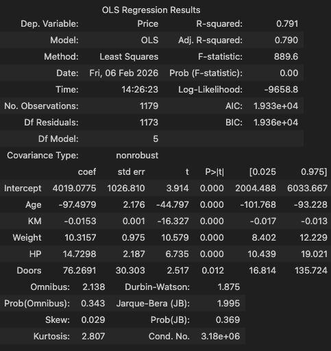

hds.stat.breushpagan(model=model)
#   Statistic	P-Value	  F-Value 	F P-Value
# 0	10.220546	0.069222	2.051491	0.069082

로지스틱 회귀

로지스틱 회귀의 개요

• 목표변수가 범주형일 때 사용하는 알고리즘
• 목표변수를 입력변수 간 선형결합으로 표현
  • 입력변수마다 목표변수에 영향을 미치는 크기를 제시
  • 해석하기 쉬운 모형으로 분류 모형에서 많이 사용
• 0 또는 1인 목표변수를 0~1 사이의 실수로 추정
  • 분류 기준점을 설정하여 추정 확률을 추정값으로 변환

로지스틱 회귀의 기본 가정

• 입력변수와 목표변수 간의 관계를 로그 오즈(로짓 함수)로 표현
  • 입력변수의 선형결합은 $-\infty$ ~ $\infty$
  • 목표변수가 이항분포를 따를 때 값을 0~1이 되도록 로짓 변환
    • $logit(p) = \ln(\frac{p}{1-p})$
• 관측값은 독립성을 유지해야 함
• 잔차의 정규성 및 등분산성 가정 X

로지스틱 회귀 프로세스

탐색적 데이터 분석 → 목표-입력변수 관계 확인 → 회귀계수 추정(가능도 방법 GLM)
→ 유의성 검정(모형, 계수) → 다중공선성 해결(분산팽창지수) → 오즈비 확인(모형 해석)

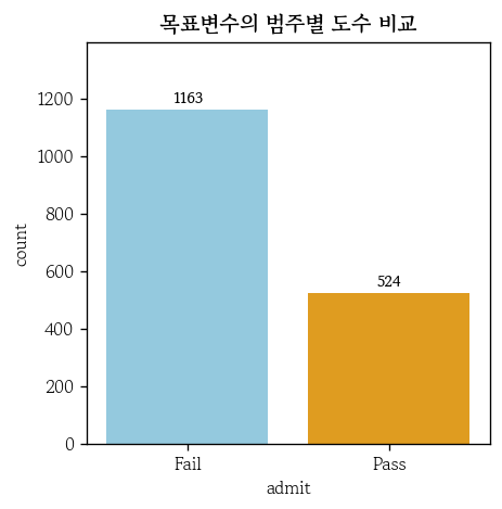
• 목표변수 도수 확인

hds.plot.bar_freq(
    data=df, x='admit', palette=['skyblue', 'orange']
)

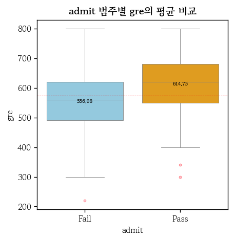
• 입력변수와 관계 확인

hds.plot.box_group(
    data=df, x='admit', y='gre',
    palette=['skyblue', 'orange']
)

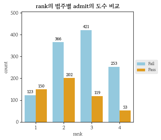
hds.plot.bar_dodge_freq(
    data=df, x='rank', g='admit',
    palette=['skyblue', 'orange']
)

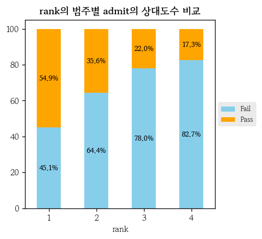
hds.plot.bar_stack_freq(
    data=df, x='rank', g='admit',
    palette=['skyblue', 'orange']
)

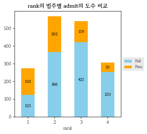
hds.plot.bar_stack_prop(
    data=df, x='rank', g='admit',
    palette=['skyblue', 'orange']
)

t-검정

pd.pivot_table(
    data=df, index='admit', values='gre',
    aggfunc=['count', 'mean', 'std'], margins=True
).round(2)
#       count	mean	std
#       gre	gre	gre
# admit			
# Fail	1163	556.08	96.36
# Pass	524	614.75	88.92
# All	1687	574.30	97.92

pg.normality(data=df, dv='gre', group='admit')
#       W	        pval	    normal
# admit			
# Fail	0.990857	0.000001	False
# Pass	0.992274	0.008138	False

pg.homoscedasticity(data=df, dv='gre', group='admit')
#         W	        pval	    equal_var
# levene	3.596208	0.058082	True

y1 = df.loc[df['admit'].eq('Fail'), 'gre']
y2 = df.loc[df['admit'].eq('Pass'), 'gre']
pg.ttest(x=y1, y=y2, correction=False)

교차분석

pd.crosstab(index=df['rank'], columns=df['admit'], margins=True, normalize='index')
# admit	Fail	Pass
# rank		
# 1	0.450549	0.549451
# 2	0.644366	0.355634
# 3	0.779630	0.220370
# 4	0.826797	0.173203
# All	0.689389	0.310611

pg.chi2_independence(data=df, x='rank', y='admit')[2]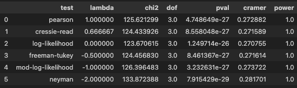

범주형 입력변수의 더미 변수 변환

df = pd.get_dummies(
    data=df, columns=['rank', 'admit'],
    prefix=['rank', None],
    dtype=int, drop_first=True
)
# gre	gpa	rank_2	rank_3	rank_4	Pass
# 0	380.0	3.61	0	1	0	0
# 1	660.0	3.67	0	1	0	1
# 2	800.0	4.00	0	0	0	1
# 3	640.0	3.19	0	0	1	1
# 4	520.0	2.93	0	0	1	0

범주형 입력변수의 더미 변수 변환

yvar = 'Pass'
X = df.drop(columns=yvar)
y = df[yvar].copy()
display(X)
display(y)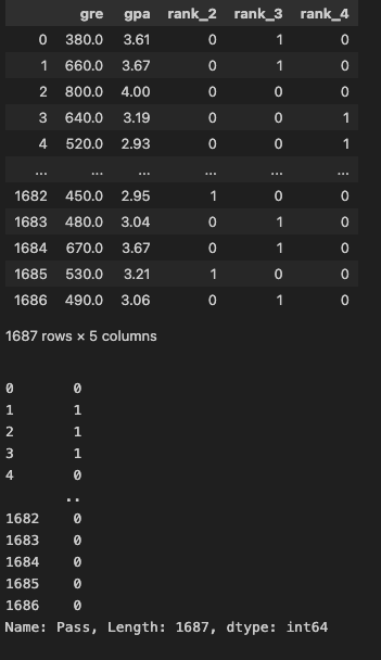

추정 확률 설정

• 입력변수 행렬 X가 주어졌을 때 목표변수가 1일 확률을 p, 0일 확률을 1-p로 설정
  • $p = P(y = 1 | X)$
  • $1-p = P(y = 0 | X)$
• 모든 관측값에 대해 p를 1에 가깝게 추정하는 문제로 변환

오즈

• 실패 확률 대비 성공 확률의 배수
  • $\frac{p}{1-p}$

로짓

• 오즈에 로그를 씌운 것을 로그 오즈 또는 로짓이라고 함
  • 로짓을 알면 확률을 계산할 수 있음

로짓 변환

• 로짓 함수와 시그모이드 함수는 역함수 관계
  • 시그모이드 : $\frac{1}{1+e^{-logit(p)}}$
• 로짓은 확률의 로그 오즈를 의미
  • 입력변수의 선형결합과 같다고 가정
• 확률과 선형결합을 연결할 수 있으므로, 확률 추정 문제로 적용 가능

최대가능도 추정법

• 서로 독립적인 사건이 함께 발생할 확률은 모두 곱함
• 양변에 자연로그를 씌우면 곱셈을 덧셈으로 변형

로지스틱 회귀 모형의 가능도 함수

• y = 0, p = 1-p
• y = 1, p = p
• $\prod_{i=1}^{n}p_{i}^{y_i}(1-p_i)^{1-y_i}$

로지스틱 회귀계수 추정 : 최대가능도 추정법

• $\ln L(\beta|X,y)$
• 이 함수를 최대로 만드는 회귀계수 $\beta$ 를 추정

로지스틱 회귀 적합 함수

• 목표변수는 이항분포를 따름
• 일반화 선형 모형(GLM)으로 적합

model = hds.stat.glm(X=X, y=y)
model.summary()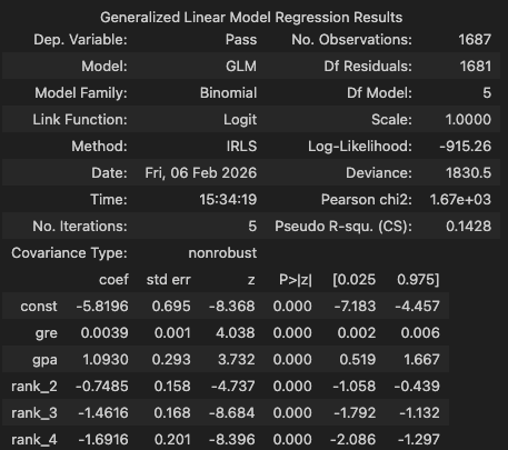

• Deviance : 모형 검정(카이제곱)
• Pseudo R-squ : 유사 계수

로지스틱 회귀 모형의 유의성 검정

• 입력변수를 추가한 residual 모형과 입력변수가 없는 null 모형 간 유의한 차이가 있는지 여부 확인
• 두 모형의 이탈도 차이로 카이제곱 검정을 실행
  • 이탈도는 작을수록 로지스틱 회귀 모형의 성능이 좋다는 것
  • 두 모형의 성능 차이가 클수록 이탈도의 차이가 증가
  • 검정통계량의 자유도는 두 모형의 자유도 차이(입력변수의 개수)로 지정

로지스틱 회귀 모형의 유의성 검정

• 검정통계량과 자유도로 유의확률을 계산

devGap = model.null_deviance - model.deviance
devGap
# np.float64(259.97760909804174)

dofGap = model.df_model
dofGap
# np.int64(5)

로지스틱 회귀계수의 유의성 검정

• 유의성 검정은 z-검정 또는 Wald 검정을 이용

1 - stats.chi2.cdf(x=devGap, df=dofGap)
# np.float64(0.0)

다중공선성 확인

• 분산팽창지수가 10 이상인 입력변수가 2개 이상 있다면 분산팽창지수가 최댓값인 입력변수 하나만 삭제 → 회귀 모형 다시 적합 후 분산팽창지수 재확인
  

오즈비

• $odds = \frac{p}{1-p}$
• 오즈비는 두 오즈의 비율
  • $e^{\beta_i}$
• 오즈를 알면 성공 확률을 계산할 수 있음
  • $p=\frac{odds}{1+odds}$
• 오즈비는 확률 자체의 변화가 아닌 오즈의 비율 변화

회귀계수를 자연상수가 밑인 지수변환 → 오즈비 얻음
오즈비는 해당 변수가 1 증가할 때 합격 오즈가 몇배인지 나타낸 값
합격 오즈를 알면 확률을 얻을 수 있음

마치며

내일 ADsP 시험을 보고 와서 이번 통계 파트에 대해 쭉 정리를 해봐야 될 것 같다.